Simple Linear Regression
Group Outlines Due
- Project Outlines due April 3rd
- Structure:
- Introduction and Motivation
- Data
- How easily available is it?
- Did you decide to use an alternative dataset?
- Methods
- What does the paper use?
- How available is replication code?
- Describe what the method is doing
- Additions/Extensions
What will we cover?
- What is a regression?
- Why does econometrics use regressions so much?
- How do we interpret regression results?
- What are the assumptions behind regressions?
- How do we estimate regressions?
- How do we solve for the OLS estimator?
What is a regression?
- Regressions come from the idea of “regressions to the mean”
- The idea that extreme values tend to be followed by more moderate values
- “Regression towards mediocrity in hereditary stature”
- Francis Galton observed that tall parents tend to have children who are shorter than them, and short parents tend to have children who are taller than them.
- So it seems that “extreme” characteristics tend to “regress” towards the average in the next generation.
What is a regression?
- Some examples of this are:
- Students who score extremely high or low on a test tend to score closer to the average on a subsequent test.
- Athletes who perform exceptionally well in their first year often see a decline in performance in their second year.
- Stock prices that experience extreme fluctuations often revert to their average levels over time.
- The sophomore slump: students who do very well in their first year of college often see a decline in performance in their second year.
What is a regression?
- Galton coined the term “regression to the mean” and developed the simple linear regression model.
- Nowadays, though, the term “regression” refers to a statistical method used to model the relationship between a dependent variable and one or more independent variables.
Why do we use regressions?
- Linear regression is used extensively in econometrics
- This can be for several reasons:
- It is relatively simple to understand and implement.
- The results are easy to interpret.
- It often provides a good approximation of the relationship between variables, even when the true relationship is not linear.
It is relatively simple to understand and implement.
- The linear regression model assumes a linear relationship between the dependent variable and the independent variables.
- The a simple regression model can be expressed mathematically as:
\[ Y = b_0 + b_1 X + e \]
Where: - \(Y\) is the dependent variable. - \(X\) is the independent variable. - \(b_0\) is the intercept. - \(b_1\) is the slope coefficient. - \(u\) is the error term.
- You can think of the coefficients as the parameters that define the line that best fits the data.
The results are easy to interpret.
- The coefficients in a linear regression model have a straightforward interpretation.
- For example, in the simple regression model above, \(b_1\) represents the change in the dependent variable \(Y\) for a one-unit increase in the independent variable \(X\), holding all other factors constant.
- This makes it easy to understand the impact of each independent variable on the dependent variable.
It often provides a good approximation of the relationship between variables, even when the true relationship is not linear.
- This is a little harder to explain, so let’s start with: conditional expectations
- Recall the conditional expectation:
\[ E[Y|X] = \int y f(y|X) dy \]
Mean Independence
- An incredibly important concept and assumption in econometrics is mean independence.
\[ E(\epsilon|X) = E(\epsilon) \]
- If this equation holds, then we say that \(u\) is mean independent of \(X\).
- This means that once we know \(X\), we don’t learn anything new about the expected value of \(u\).
- This is a weaker condition than full independence, which would require that the entire distribution of \(u\) is independent of \(X\).
Example
- Let’s say we are studying the relationship between wages and education level.
- Let \(Y\) be the wage and \(X\) be the years of education.
- Mean independence would imply that \(E(Y|X=8)=E(Y|X=12)=E(Y|X=16)\).
- So this is saying that your expected wage is the same regardless of whether you have 8, 12, or 16 years of education.
- Is that a good assumption?
Example
- Let’s say that instead, we have \(u\) be unobserved ability.
- Mean independence would imply that \(E(u|X=8)=E(u|X=12)=E(u|X=16)\).
- So this is saying that your expected ability is the same regardless of whether you have 8, 12, or 16 years of education.
- Is that a good assumption?
Example
- Can you tell me a story where this assumption might hold?
- What theory of ability might lead us to believe this?
- Can you tell me a story where this assumption might fail?
- What theory of ability might lead us to believe this assumption fails?
The Conditional Expectation Function
- But let’s say that we are willing to make that mean independence assumption.
- And lets add an assumption, that one average ability it 0. This is called a normalization.
\[ E(\epsilon) = 0 \]
- Then what you get is a key identifying assumption in econometrics:
\[ E(\epsilon|X)=0 \]
- This is called the zero conditional mean assumption.
\[ Y = E(Y|X) + \epsilon \]
- This is called the conditional expectation function (CEF).
What is the point?
- What was the point of all that setup?
- We now have two objects to think about:
\[ Y = b_0 + b_1 X + e \]
and
\[ Y = E(Y|X) + \epsilon =?= \beta_0 + \beta_1 X + \epsilon \]
- This first is a linear regression line, or the best fit line, which we will call OLS.
- The second is the true population regression function.
- The CEF need not be linear, but if it is, then we can write it as \(\beta_0 + \beta_1 X\). But we’ll see that even if it isn’t, we are still in good shape.
- If we can estimate \(b_0\) and \(b_1\) to be equal to \(\beta_0\) and \(\beta_1\), then we have causally identified the effect of \(X\) on \(Y\).
The Conditional Expectation Function Decomposition
- Note that \(Y = E(Y|X) + \epsilon\) actually needs to be proven.
- This is actually a pretty powerful idea.
- It says that any random variable \(Y\) can be decomposed into two parts:
- A part that is explained by \(X\) (the conditional expectation)
- A part that is not explained by \(X\) (the error term)
- It’s only true if:
- \(E(\epsilon|X) = 0\) (zero conditional mean assumption)
- \(\epsilon\) is uncorrelated with any function of \(X\) (which follows from 1)
Proof of point 1
\[ \begin{aligned} E\left(\varepsilon_i \mid x_i\right) & =E\left(y_i-E\left(y_i \mid x_i\right) \mid x_i\right) \\ & =E\left(y_i \mid x_i\right)-E\left(y_i \mid x_i\right) \\ & =0 \end{aligned} \]
Proof of point 2
Your turn, assume that you have some function \(X\), \(h(X)\).
\(E\left(h\left(x_i\right) \varepsilon_i\right)=E\left\{h\left(x_i\right) E\left(\varepsilon_i \mid x_i\right)\right\}\)
Other properties
- The CEF is the best predictor of \(Y\) given \(X\) in the mean squared error sense, so regardless of what function of \(X\) you are using.
- ANOVA: \(Var(Y) = Var(E(Y|X)) + E(Var(Y|X))\)
- The total variance of \(Y\) can be decomposed into the variance explained by \(X\) and the variance not explained by \(X\).
Again.. what’s the point?
- All of this lead up was to motivate one thing…
- Applied econometricians often use linear models.
- But we can all agree that the world is not linear.
- The true data-generating process and population model is incredibly complicated.
- So why do we use linear models so much?
Linear Regression, the CEF and Linearity
- If the population CEF actually, is linear in \(X\), then the linear regression model is correctly specified.
- If the population CEF is not linear in \(X\), then the linear regression model is misspecified. But! The linear regressions model still provides the best linear approximation to the true CEF.
- So even if the true relationship between \(X\) and \(Y\) is not linear, the linear regression model can still provide a useful first-order approximation of that relationship.
What is a best fit line?
- How do we find the best fit line?
- What is the best fit line?
- How do we obtain it?
- It depends on what loss function we use.
- We use mean squared error (MSE) as our loss function.
- How well does it fit the data? How much of the overall variation of y is explained by x?
- Different samples would yield different lines
- So that means that b0 and b1 are random variables and have distributions…
- But hat also means we can construct confidence intervals and do hypothesis tests!
Estimating OLS
- How do we estimate \(b_0\) and \(b_1\)?
- We use the method of Ordinary Least Squares (OLS).
- This means that we minimize the mean squared error (MSE) between the observed values of \(Y\) and the predicted values of \(Y\) from the regression line.
- What is a residual?
- A residual is the difference between the observed value of the dependent variable and the value predicted by the regression model.
\[ e_i = Y_i - b_0 - b_1 X_i \]
- for each observation \(i\) in our sample.
Estimating OLS
Note the two assumptions we made earlier:
- Mean independence: \(E(\epsilon|X) = E(\epsilon)\)
- Normalization: \(E(\epsilon) = 0\)
We can derive the OLS estimators for \(b_0\) and \(b_1\) using these assumptions.
From here, there are two things we can say further:
Mean independence gives us that \(E(X \epsilon) = 0\)
From there we can also say that \(Cov(X, \epsilon) = 0\)
Why?
- Recall the Law of Iterated Expectations:
\[ E(X \epsilon) = E[E(X \epsilon | X)] = E[X E(\epsilon | X)] = E[X \cdot 0] = 0 \]
- This brings us to two important results:
\[ E(\epsilon) = E(y - \beta_0 - \beta_1 X) = 0 \]
and
\[ E(X \epsilon) = E[X(y - \beta_0 - \beta_1 X)] = 0 \]
- Note that these are all in population terms.
Estimating OLS
From here, we can derive the OLS estimators for \(b_0\) and \(b_1\).
But we need one more thing first: sample analogues.
Sample analogues are the sample counterparts of population parameters.
We don’t have access to the population data, but we do have access to sample data.
So we can replace the population expectations with sample averages:
\[ \frac{1}{n} \sum_{i=1}^{n} Y_i - b_0 - b_1 X_i = 0 \]
and
\[ \frac{1}{n} \sum_{i=1}^{n} X_i (Y_i - b_0 - b_1 X_i) = 0 \]
Now solve the system of equations for \(b_0\) and \(b_1\).
- Do the algebra to solve for b0 and b1
THe work:
From the first equation: \[ b_0 = \bar{Y} - b_1 \bar{X} \]
and from the second:
\[ \sum_{i=1}^{n} X_i Y_i - b_0 \sum_{i=1}^{n} X_i - b_1 \sum_{i=1}^{n} X_i^2 = 0 \]
Plugging in for b0:
\[ \begin{aligned} \sum_{i=1}^n x_i\left[y_i-\left(\bar{y}-\widehat{\beta_1} \bar{x}\right)-\widehat{\beta_1} x_i\right] & =0 \\ \sum_{i=1}^n x_i\left(y_i-\bar{y}\right) & =\widehat{\beta_1}\left[\sum_{i=1}^n x_i\left(x_i-\bar{x}\right)\right] \end{aligned} \]
which is equivalent to:
\[ \sum_{i=1}^n\left(x_i-\bar{x}\right)\left(y_i-\bar{y}\right)=\widehat{\beta_1}\left[\sum_{i=1}^n\left(x_i-\bar{x}\right)^2\right] \]
Why?
\[ \begin{aligned} \sum_{i=1}^n\left(x_i-\bar{x}\right)\left(y_i-\bar{y}\right) & =\sum_{i=1}^n x_i\left(y_i-\bar{y}\right) \\ & =\sum_{i=1}^n\left(x_i-\bar{x}\right) y_i=\sum_{i=1}^n x_i y_i-n(\bar{x} \bar{y}) \end{aligned} \]
Estimating OLS
- So in the end what we have is:
\[ b_1 = \frac{\sum_{i=1}^{n} (X_i - \bar{X})(Y_i - \bar{Y})}{\sum_{i=1}^{n} (X_i - \bar{X})^2} \]
which can be rewritten as:
\[ b_1 = \frac{\text{Sample Cov(X,Y)}}{\text{Sample Var(X)}} \]
and
\[ b_0 = \bar{Y} - b_1 \bar{X} \]
Some definitions:
- The fitted values are the predicted values of \(Y\) from the regression line:
\[ \hat{Y}_i = b_0 + b_1 X_i \]
- The residuals are the differences between the observed values of \(Y\) and the fitted values:
\[ e_i = Y_i - \hat{Y}_i \]
OLS Residuals
What if we go ahead and try to quantify the error in our predictions?
The residual ALWAYS sum to zero by construction:
There’s several ways to see this:
- If you’ve taken calculus, note that the first order condition for minimizing the sum of squared residuals with respect to b0 is:
\[ \frac{\partial}{\partial b_0} \sum_{i=1}^{n} e_i^2 = -2 \sum_{i=1}^{n} e_i = 0 \]
- \(b_0\) is chosen so that the fitted line passes through the mean of the data, which forces the residuals to “balance out” around zero.
- You can sort of see it from the perspective that it “demeans” the data.
OLS Residuals
- This also means that:
\[ Cov(\hat{Y_i}, e_i) = 0 \]
Why?
Recall that the covariance is defined as: \[ Cov(X, Y) = E[(X - E(X))(Y - E(Y))] \]
So if we let \(X = \hat{Y_i}\) and \(Y = e_i\), then we have:
\[ Cov(\hat{Y_i}, e_i) = E[(\hat{Y_i} - E(\hat{Y_i}))(e_i - E(e_i))] \]
- But we know that \(E(e_i) = 0\), so this simplifies to:
\[ Cov(\hat{Y_i}, e_i) = E[(\hat{Y_i} - E(\hat{Y_i}))e_i] \]
\[ = E[\hat{Y_i} e_i] - E[\hat{Y_i}] E[e_i] \]
- Why can we make that move?
- What does that move mean?
The CLRF Assumptions
A0: Linearity
The model can be written as:
\[ Y = b_0 + b_1 X + \epsilon \]
A1: \(E(\epsilon) = 0\)
A2: \(E(\epsilon|X) = 0\)
Which also means what, when we include A1?
A3: Homoskedasticity
\[ Var(\epsilon|X) = \sigma^2 \]
A4: No autocorrelation
\[ Cov(\epsilon_i, \epsilon_j|X) = 0 \text{ for } i \neq j \]
Similarly, we can also say:
\[ E(\epsilon_i \epsilon_j|X) = 0 \text{ for } i \neq j \]
Why?
A5: \(\epsilon\) is normally distributed (for small samples)
Goodness of Fit
- Since OLS is a model that approximates the relationship between \(X\) and \(Y\), we might want to know how well it fits the data.
- One common measure of goodness of fit is the R-squared (\(R^2\))
Goodness of Fit
- More definitions!
- Total Sum of Squares (TSS)
- Explained Sum of Squares (ESS)
- Residual Sum of Squares (RSS/SSR)
- All comes from decomposing the total variation in \(Y\).
\[ Y = \hat{Y} + \hat{u} \]
\[ TSS = \sum_{i=1}^{n} (Y_i - \bar{Y})^2 \]
\[ ESS = \sum_{i=1}^{n} (\hat{Y}_i - \bar{Y})^2 \]
\[ RSS/SSR = \sum_{i=1}^{n} (Y_i - \hat{Y}_i)^2 \]
Goodness of Fit
- The ESS and RSS sum to the TSS
\[ TSS = \sum_{i=1}^{n} (Y_i - \bar{Y})^2 \]
\[ = \sum_{i=1}^{n} (\hat{Y}_i - \hat{Y} + \hat{Y} - \bar{Y})^2 \]
\[ = \sum_{i=1}^{n} (\hat{Y}_i - \bar{Y})^2 + \sum_{i=1}^{n} (Y_i - \hat{Y}_i)^2 + 2 \sum_{i=1}^{n} (\hat{Y}_i - \bar{Y})(Y_i - \hat{Y}_i) \]
- The last term is zero
- Why?
What is \((Y_i - \hat{Y}_i)\)? The residual, \(e_i\).
So what is this term really calculating?
\[ \sum_{i=1}^{n} (\hat{Y}_i - \bar{Y}) e_i \]
- This is the covariance between the fitted values and the residuals, multiplied by \(n-1\)
- But we know that the covariance between the fitted values and the residuals is zero!
- Why?
Goodness of Fit
So now we know that:
\[ TSS = ESS + RSS \]
- What are these quantities?
- These are sample variances, really…
\[ \frac{1}{n} \sum_{i=1}^{n} (Y_i - \bar{Y})^2 = \frac{1}{n} \sum_{i=1}^{n} (\hat{Y}_i - \bar{Y})^2 + \frac{1}{n} \sum_{i=1}^{n} (Y_i - \hat{Y}_i)^2 \]
TSS -> Sample Variance of Y
ESS -> Sample Variance of Fitted Values
RSS -> Sample Variance of Residuals
So we can write:
\[ Var(Y) = Var(\hat{Y}) + Var(e) \]
Goodness of Fit
- If we want to understant how well our model fits the data, an intuitive way to do so would be to ask the question:
How much of the total variation in \(Y\) is explained by the model (\(X\))?
- This is exactly what R-squared (\(R^2\)) measures:
\[ R^2 = \frac{ESS}{TSS} = 1 - \frac{RSS}{TSS} \]
- One is in terms of explained variation, the other in terms of unexplained variation.
Goodness of Fit
- Why is it named \(R^2\)?
- The correlation coefficient is sometimes know as \(R\).
- Remember that correlation is between -1 and 1.
\[ R = \frac{Cov(X,Y)}{\sqrt{Var(X) Var(Y)}} \]
- It turns out that in simple linear regression, the square of the correlation coefficient between \(X\) and \(Y\) is equal to the R-squared value from the regression.
- So \(R^2\) is the square of the correlation coefficient between the independent variable and the dependent variable in a simple linear regression.
Goodness of Fit
- So what does \(R^2\) tell us?
- \(R^2\) is between 0 and 1.
- An \(R^2\) of 0 means that the model does not explain any of the variation in \(Y\).
- An \(R^2\) of 1 means that the model explains all of the variation in \(Y\).
- In general, a higher \(R^2\) indicates a better fit of the model to the data.
- It does not imply causation.
- High fit of the data doesn’t mean that X causes Y.
- \(R^2\) is not a good measure across different \(Y\) variables.
- But it is good when thinking about different \(X\) variables for the same \(Y\) variable.
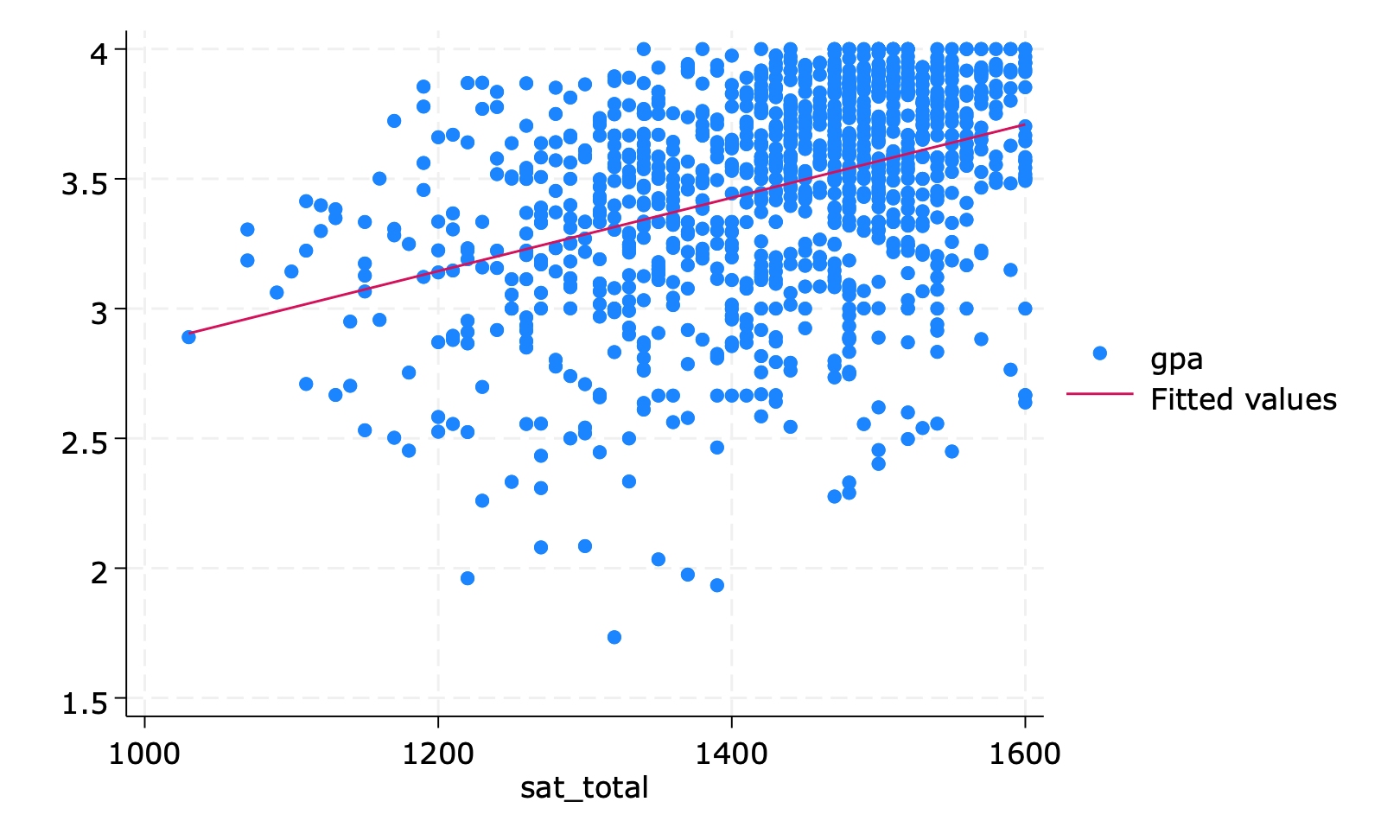
Goodness of Fit
Example in Stata