Continuous Probability Distributions

EC031-S26

Agenda

• Uniform Probability Distribution
• Normal Probability Distribution
• Normal Approximation of Binomial Probabilities
• Exponential Probability Distribution

Continuous Probability Distributions

• A continuous random variable can assume any value in an interval on the real line or in a collection of intervals.
• It is not possible to talk about the probability of the random variable assuming a particular value.
• Instead, we talk about the probability of the random variable assuming a value within a given interval.

Continuous Probability Distributions

The probability of the random variable assuming a value within some given interval from x1 to x2 is defined to be the area under the graph of the probability density function between x1 and x2.

Uniform Probability Distribution

• A random variable is uniformly distributed whenever the probability is proportional to the interval’s length.
• The uniform probability density function is:

\[ f(x)= \begin{cases} \frac{1}{b - a} \text{ for } a \leq x \leq b \\ 0 \text{ otherwise} \end{cases} \]

Uniform Probability Distribution

• The expected value of x is \(E(x) = \frac{(a + b)}{2}\).
• The variance of x is \(Var(x) = \frac{(b – a)^2}{12}\).
• Why?

viewof a = Inputs.range([0, 10], {value: 5, step: 0.1, label: "Uniform Distribution: a"});
viewof b = Inputs.range([0, 10], {value: 8, step: 0.1, label: "Uniform Distribution: b"});
Plot.plot({
  marks: [
    Plot.line(d3.range(a, b, 0.01).map(x => ({x, y: 1 / (b - a)})), {x: "x", y: "y"})
  ],
  x: {label: "x"},
  y: {label: "Probability Density"}
})

For continuous random variables, the expected value is defined as:

\[ E(x) = \int_{-\infty}^{\infty} x f(x) \, dx \]

In this case, the endpoints go from a to b since the probability density function is zero outside this interval.

Calculating the expected value:

\[ E(x) = \int_{a}^{b} x \cdot \frac{1}{b - a} \, dx = \frac{1}{b - a} \int_{a}^{b} x \, dx = \frac{1}{b - a} \left[ \frac{x^2}{2} \right]_{a}^{b} = \frac{1}{b - a} \left( \frac{b^2}{2} - \frac{a^2}{2} \right) = \frac{b + a}{2} \]

What about variance? We can define variance as:

\[ Var(x) = E(x^2) - [E(x)]^2 \]

Why?

Variance Tricks

• Why can we define variance as \(Var(x) = E(x^2) - [E(x)]^2\)?
• This is a useful trick for calculating variance, because it allows us to calculate the variance without having to calculate the expected value of the random variable first.
• We can calculate \(E(x^2)\) and \(E(x)\) separately, and then use the formula to get the variance.
• Let’s derive this:

\[ \begin{split} Var(x) &= E[(x - E(x))^2] \\ &= E[x^2 - 2xE(x) + (E(x))^2] \\ &= E(x^2) - 2E(x)E(x) + (E(x))^2 \\ &= E(x^2) - 2(E(x))^2 + (E(x))^2 \\ &= E(x^2) - (E(x))^2 \end{split} \]

Back to the Example

Calculating \(E(x^2)\): \[ E(x^2) = \int_{a}^{b} x^2 \cdot \frac{1}{b - a} \, dx = \frac{1}{b - a} \int_{a}^{b} x^2 \, dx = \frac{1}{b - a} \left[ \frac{x^3}{3} \right]_{a}^{b} = \frac{1}{b - a} \left( \frac{b^3}{3} - \frac{a^3}{3} \right) = \frac{b^2 + ab + a^2}{3} \]

Now we can compute the variance: \[ Var(x) = E(x^2) - [E(x)]^2 = \frac{b^2 + ab + a^2}{3} - \left( \frac{b + a}{2} \right)^2 = \frac{(b - a)^2}{12} \] :::

Example

• Suppose that the time it takes to complete a task is uniformly distributed between 5 and 10 minutes.

• What is the probability that the task will take between 6 and 8 minutes?

NoteSolution

• The probability is the area under the graph of the probability density function between 6 and 8 minutes.
• The area is the length of the interval times the height of the probability density function.
• The probability is \(2 \times \frac{1}{10 - 5} = \frac{2}{5}\).

Example: Slater’s Buffet

Slater’s customers are charged for the amount of salad they take. Sampling suggests that the amount of salad taken is uniformly distributed between 5 ounces and 15 ounces. The uniform probability density function is:

\[ f(x)= \begin{cases} \frac{1}{15 - 5} \text{ for } 5 \leq x \leq 15 \\ 0 \text{ otherwise} \end{cases} \]

Example: Slater’s Buffet

What is the probability that a customer will take between 12 and 15 ounces of salad?

Example: Slater’s Buffet

The expected value of x is:

\[ E(x) = \frac{(5 + 15)}{2} = 10 \]

The variance of x is:

\[ \text{Var}(x) = \frac{(15 - 5)^2}{12} = 8.33 \]

Usefulness of the Uniform Distribution

• Another way to think of the uniform distribution is that it is a “flat prior.”
• In the absence of any other information, we can assume that any outcome is equally likely, just \(\frac{1}{b - a}\).
  • All you need is some information on some minimum and maximum values.
• It’s also a way to express a simple way to randomize, giving each outcome equal weight.

Area as a Measure of Probability

• The area under the graph of f(x) and probability are identical.
• This is valid for all continuous random variables.
• The probability that x takes on a value between some lower value \(x_1\) and some higher value \(x_2\) can be found by computing the area under the graph of \(f(x)\) over the interval from \(x_1\) to \(x_2\).

Warning

What is the probability of a continuous random variable taking on a specific value, say \(x = c\)?

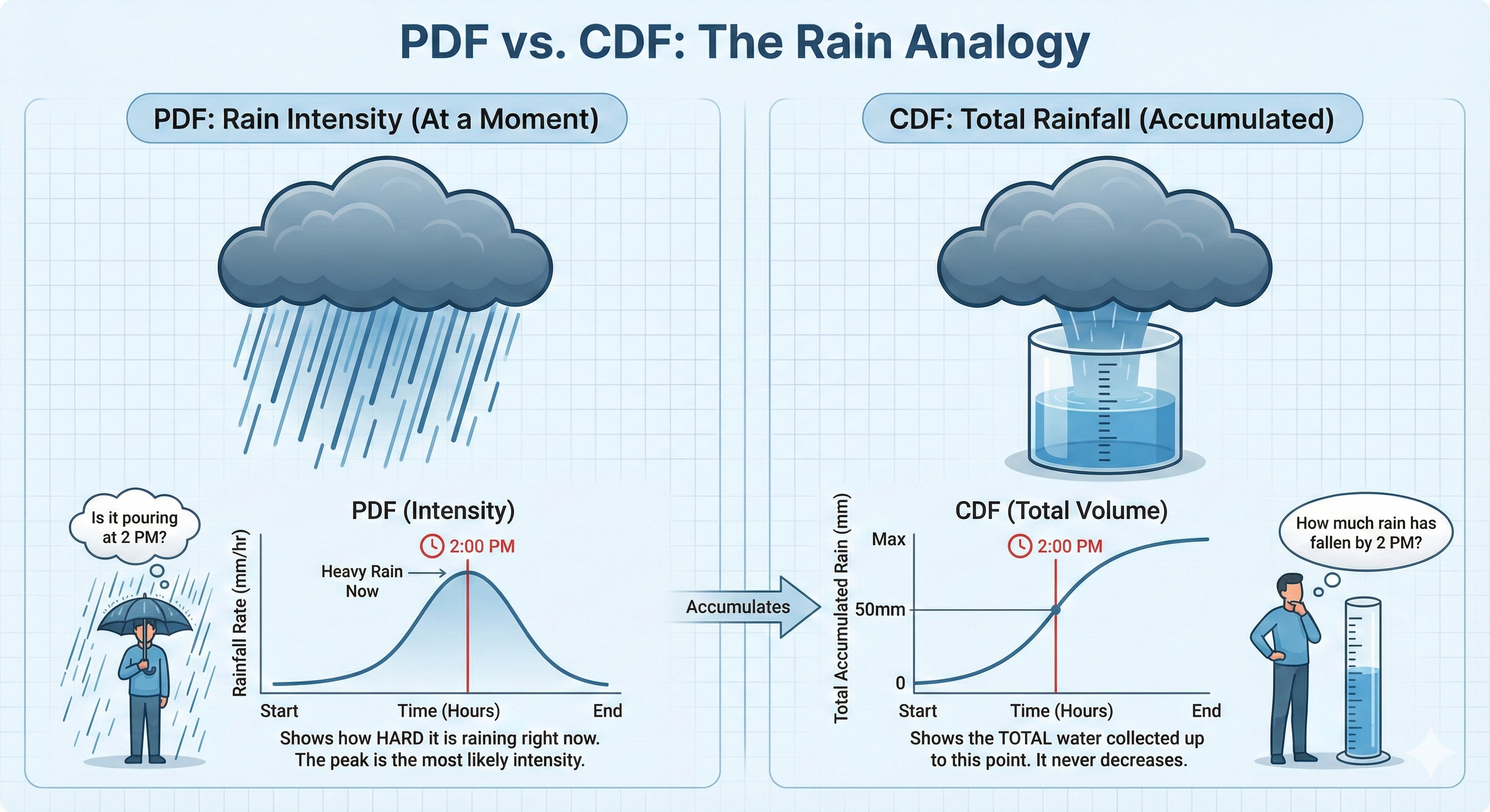
Cumulative Probability

• Sort of review: What is a cumulative probability distribution, vs. a probability distribution?
  • We talked about this with discrete random variables.
• The cumulative probability distribution gives the probability that the random variable is less than or equal to a certain value.
• For continuous random variables, it is the area under the probability density function up to that value.
• But the PDF function, itself, shows where probability might be concentrated.

Cumulative Probability

What is the CDF of a Uniform Random Variable?

• What would that look like?
• Let’s draw it out.

I want to draw this on the board. We start with a uniform distribution, and then go through the process of calculating cumulative probabilities for different values of x.

• start by drawing a uniform distribution between a and b.
• then, for a value x0 between a and b, we calculate the area under the curve from a to x0. This area represents the cumulative probability P(X ≤ x0).
• Just calculate the area of the rectangle.

\[ F(x) = \begin{cases} 0 \text{ for } x < a \\ \frac{x - a}{b - a} \text{ for } a \leq x \leq b \\ 1 \text{ for } x > b \end{cases} \]

Other Continuous Probability Distributions

• There are many other continuous probability distributions.
• They are used to model different types of phenomena.
• If the uniform distribution gives us a situation with a lot of uncertainty about outcomes, other distributions make more specific assumptions about the nature of the random variable, and which outcomes are more likely.

Exponential Probability Distribution

• The exponential probability distribution is useful in describing the time it takes to complete a task.
• The exponential random variables can be used to describe:
  • Time between vehicle arrivals at a toll booth
  • Time required to complete a questionnaire
  • Distance between major defects in a highway
• In waiting line applications, the exponential distribution is often used for service time.

Exponential Probability Distribution

• A property of the exponential distribution is that the mean and standard deviation are equal.
• The exponential distribution is skewed to the right.

\[ f(x) = \frac{1}{\lambda} e^{-\frac{1}{\lambda} x} \]

\[ P(x \leq x_0) = 1 - e^{-\frac{1}{\lambda} x_0} \]

where \(x_0\) is the value of the random variable and \(\lambda\) is the mean of the random variable.

Cumulative Probability vs Probability Density

viewof lambda_demo = Inputs.range([0.1, 5], {value: 1, step: 0.1, label: "Lambda"});
viewof t_val = Inputs.range([0, 10], {value: 2, step: 0.1, label: "t"});

Plot.plot({
  height: 200,
  grid: true,
  x: {domain: [0, 10], label: "x"},
  y: {label: "PDF f(x)"},
  marks: [
    Plot.areaY(d3.range(0, t_val, 0.01).map(x => ({x, y: lambda_demo * Math.exp(-lambda_demo * x)})), {x: "x", y: "y", fill: "steelblue", fillOpacity: 0.3}),
    Plot.line(d3.range(0, 10, 0.01).map(x => ({x, y: lambda_demo * Math.exp(-lambda_demo * x)})), {x: "x", y: "y", stroke: "steelblue"}),
    Plot.ruleX([t_val], {stroke: "red", strokeDasharray: "4"})
  ]
})

Plot.plot({
  height: 200,
  grid: true,
  x: {domain: [0, 10], label: "x"},
  y: {label: "CDF F(x)", domain: [0, 1]},
  marks: [
    Plot.line(d3.range(0, 10, 0.01).map(x => ({x, y: 1 - Math.exp(-lambda_demo * x)})), {x: "x", y: "y", stroke: "orange"}),
    Plot.ruleX([t_val], {stroke: "red", strokeDasharray: "4"}),
    Plot.dot([{x: t_val, y: 1 - Math.exp(-lambda_demo * t_val)}], {x: "x", y: "y", fill: "red"}),
    Plot.text([{x: t_val, y: 1 - Math.exp(-lambda_demo * t_val)}], {x: "x", y: "y", text: d => `P(X ≤ ${t_val.toFixed(1)}) = ${(1 - Math.exp(-lambda_demo * t_val)).toFixed(2)}`, dy: -10, fill: "red"})
  ]
})

Example: Time Between Calls

The time between calls to a customer service center is exponentially distributed with a mean of 10 minutes.

What is the probability that the time between calls is less than 5 minutes?

NoteSolution

\[ P(x \leq 5) = 1 - e^{-\frac{1}{10} \times 5} = 1 - e^{-0.5} = 1 - 0.6065 = 0.3935 \]

Example: Al’s Full-Service Pump

The time between arrivals of cars at Al’s full-service gas pump follows an exponential probability distribution with a mean time between arrivals of 3 minutes. Al would like to know the probability that the time between two successive arrivals will be 2 minutes or less.

Relationship between the Poisson and Exponential Distributions

Normal Probability Distribution

• The normal probability distribution is widely used in statistical inference.
• It has been used in a wide variety of applications including:
  • Heights of people
  • Amounts of rainfall
  • Test scores
  • Scientific measurements

Abraham de Moivre, a French mathematician, published The Doctrine of Chances in 1733.

He derived the normal distribution. But it has been independently found by several mathematicians.

Normal Probability Distribution

\[ f(x) = \frac{1}{\sqrt{2\pi}\sigma}e^{-\frac{1}{2}(\frac{x - \mu}{\sigma})^2} \]

where: - \(x\) is the value of the random variable - \(\mu\) is the mean of the random variable - \(\sigma\) is the standard deviation of the random variable - \(\pi\) = 3.14159 - \(e\) = 2.71828

viewof mean = Inputs.range([-5, 5], {value: 0, step: 0.1, label: "Normal Distribution: Mean"});
viewof stddev = Inputs.range([0.1, 5], {value: 1, step: 0.1, label: "Normal Distribution: Std Dev"});
Plot.plot({
  marks: [
    Plot.line(d3.range(-10, 10, 0.01).map(x => ({x, y: (1 / (stddev * Math.sqrt(2 * Math.PI))) * Math.exp(-0.5 * ((x - mean) / stddev) ** 2)})), {x: "x", y: "y"})
  ],
  x: {label: "x"},
  y: {label: "Probability Density"}
})

Normal Probability Distribution

The entire family of normal probability distributions is defined by its mean μ and its standard deviation σ.

The highest point on the normal curve is at the mean, which is also the median and mode.

The mean can be any numerical value: negative, zero, or positive.

The standard deviation determines the width of the curve: larger values result in wider, flatter curves.

viewof mean2 = Inputs.range([-5, 5], {value: 0, step: 0.1, label: "Normal Distribution: Mean"});
viewof stddev2 = Inputs.range([0.1, 5], {value: 1, step: 0.1, label: "Normal Distribution: Std Dev"});
Plot.plot({
  marks: [
    Plot.line(d3.range(-10, 10, 0.01).map(x => ({x, y: (1 / (stddev2 * Math.sqrt(2 * Math.PI))) * Math.exp(-0.5 * ((x - mean2) / stddev2) ** 2)})), {x: "x", y: "y"})
  ],
  x: {label: "x"},
  y: {label: "Probability Density"}
})

Normal Probability Distribution

Probabilities for the normal random variable are given by areas under the curve. The total area under the curve is 1 (0.5 to the left of the mean and 0.5 to the right).

The probability that the random variable assumes a value between \(x_1\) and \(x_2\) is the area under the curve between \(x_1\) and \(x_2\).

Normal Probability Distribution

math = require("mathjs");

viewof x1 = Inputs.range([-10, 10], {value: 0, step: 0.01, label: "a"});


Plot.plot({
    marks: [
        Plot.line(d3.range(-10, 10, 0.01).map(x => ({x, y: (1 / (stddev2 * Math.sqrt(2 * Math.PI))) * Math.exp(-0.5 * ((x - 0) / 1) ** 2)})), {x: "x", y: "y"}),
        Plot.areaY(d3.range(-10, x1, 0.01).map(x => ({x, y: (1 / (1 * Math.sqrt(2 * Math.PI))) * Math.exp(-0.5 * ((x - 0) / 1) ** 2)})), {x: "x", y: "y", fillOpacity: 0.3})
    ],
    x: {label: "x"},
    y: {label: "Probability Density"}
})

function normalCDF(x, mean, stddev) {
    return 0.5 * (1 + math.erf((x - mean) / (stddev * Math.sqrt(2))));
}

area = normalCDF(x1, 0, 1);

md`The area under the normal distribution curve for x <= ${a} is ${area.toFixed(4)}.`

Empirical Rule

• 68.26% of values within ±1 standard deviation of its mean.
• 95.44% of values within ±2 standard deviations of its mean.
• 99.72% of values within ±3 standard deviations of its mean.

Standard Normal Distribution

A random variable having a normal distribution with a mean of 0 and a standard deviation of 1 is said to have a standard normal probability distribution.

The letter z is used to designate the standard normal random variable.

Converting to a Standard Normal Distribution

\[ z = \frac{x - \mu}{\sigma} \]

where: - \(z\) is the standard normal random variable - \(x\) is the value of the random variable - \(\mu\) is the mean of the random variable - \(\sigma\) is the standard deviation of the random variable

We can think of z as a measure of the number of standard deviations x is from μ.

Example: Pep Zone

Pep Zone sells auto parts and supplies including a popular multi-grade motor oil. When the stock of this oil drops to 20 gallons, a replenishment order is placed.

The store manager is concerned that sales are being lost due to stockouts while waiting for a replenishment order.

It has been determined that demand during replenishment lead-time is normally distributed with a mean of 15 gallons and a standard deviation of 6 gallons.

The manager would like to know the probability of a stockout during replenishment lead-time. In other words, what is the probability that demand during lead-time will exceed 20 gallons?

How to Solve

Step 1: Convert the random variable to a standard normal random variable.

\[ z = \frac{x - \mu}{\sigma} = \frac{20 - 15}{6} = 0.83 \]

Step 2: Find the area under the standard normal curve to the left of \(𝑧 = 0.83\).

Step 3: Compute the area under the standard normal curve to the right of \(z = 0.83\).

Why?

Note

To get the area of the other side, we simply need to use the fact that the complement of the area to the left of \(z = 0.83\) is the area to the right of \(z = 0.83\).

Example

Using a standard normal distribution, calculate:

\[ P(0 \leq z \leq 0.83) \]

Example

If the manager of Pep Zone wants the probability of a stockout during replenishment lead-time to be no more than .05, what should the reorder point be?

Step 1: Find the z-value that cuts off an area of .05 in the right tail of the standard normal distribution by looking up the complement of the right tail area

\(1 – 0.05 = 0.95.\)

Step 2: Convert \(z_{.05}\) to the corresponding value of x.

\[ z_{.05} = 1.645 \]

\[ x = \mu + z_{.05} \times \sigma = 15 + 1.645 \times 6 = 24.87 \]

Example

By raising the reorder point from 20 gallons to 25 gallons on hand, the probability of a stockout decreases from about .20 to .05.