Descriptive Statistics
Agenda
- Measures of Location
- Measures of Variability
- Measures of Distribution Shape, Relative Location, and Detecting Outliers
- Five-Number Summaries and Box Plots
- Measures of Association Between Two Variables
- Data Dashboards: Adding Numerical Measures to Improve Effectiveness
Parameters vs. Statistics
- If the measures are computed for data from a sample, they are called sample statistics.
- If the measures are computed for data from a population, they are called population parameters.
- A sample statistic is referred to as the point estimator of the corresponding population parameter.
Measures of Location
- Mean
- Median
- Mode
- Weighted Mean
- Percentiles
- Quartiles
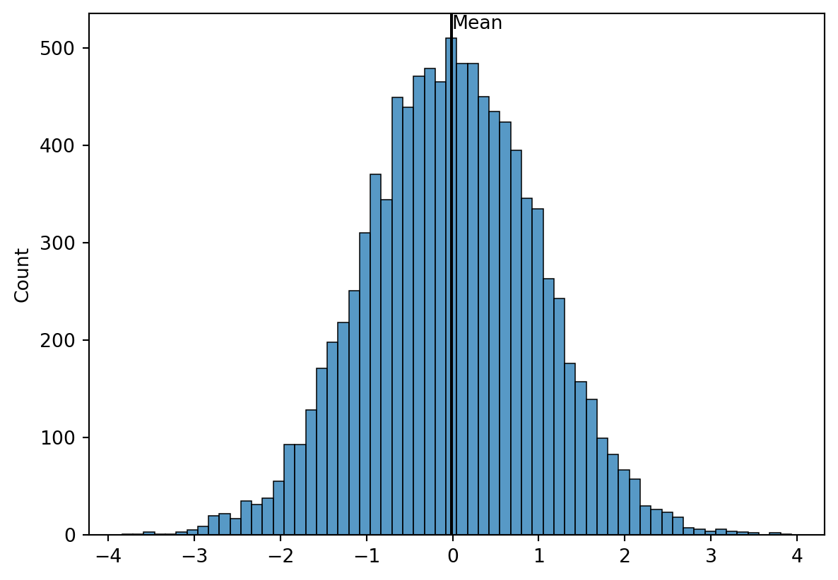
The Mean
- Perhaps the most important measure of location is the mean.
- The mean provides a measure of central location.
- The mean of a data set is the average of all the data values.
- The sample mean \(\bar{x}\) is the point estimator of the population mean, \(\mu\).
\[ \bar{x} = \frac{\sum_i^n x_i}{n} \]
Note: \(\sum_i^n x_i = x_1 + x_2 + x_3 + ... + x_n\)
Looking at the Mean
What do you see?
Example
Calculate the mean:
\(x = \{10,20,4,5\}\)
Median
- The median of a data set is the value in the middle when the data items are arranged in ascending order.
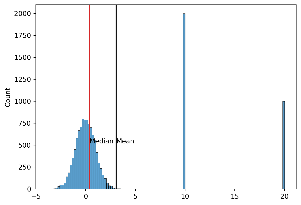
- Whenever a data set has extreme values, the median is the preferred measure of central location.
- The median is the measure of location most often reported for annual income and property value data.
- A few extremely large incomes or property values can inflate the mean.
Median
Here we have an odd number of observations: 7 observations: 26, 18, 27, 12, 14, 27, and 19. Rewritten in ascending order: 12, 14, 18, 19, 26, 27, and 27.
What is the median?
The median is the middle value in this list, so the median = 19.
Median
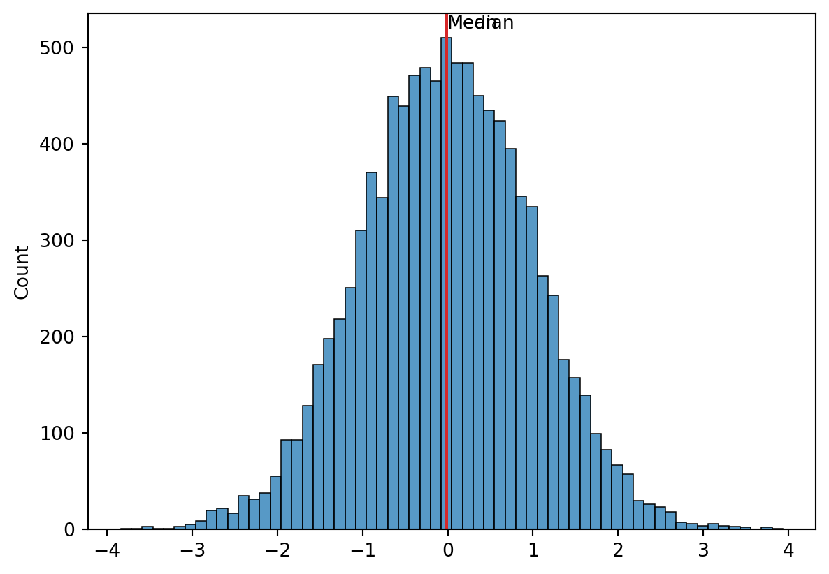
Median
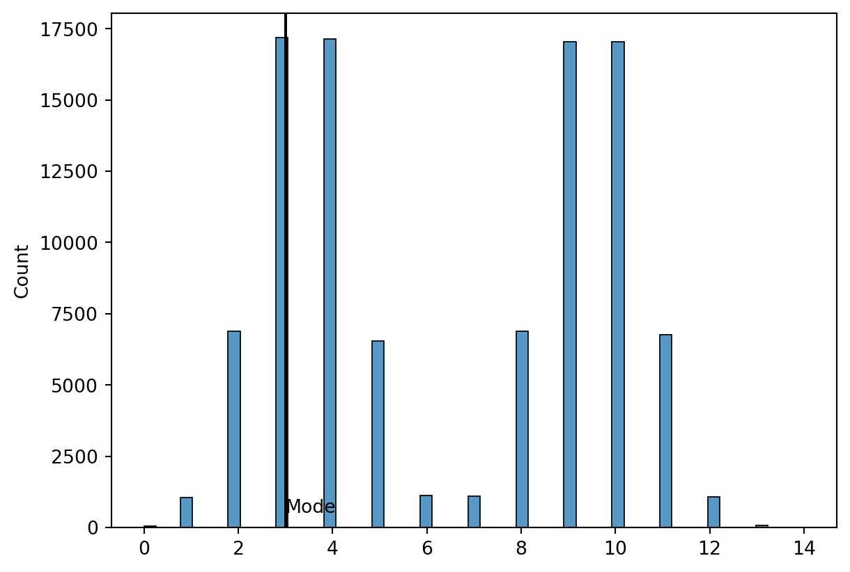
Mode
- The mode of a data set is the value that occurs with greatest frequency.
- The greatest frequency can occur at two or more different values.
- If the data have exactly two modes, the data are bimodal.
- If the data have more than two modes, the data are multimodal.
Bimodal Distributions
Weighted Means
- Weighted means make a lot more sense when you think of the mean as a weighted mean, itself.
- What assumption is the simple mean making when divide by \(N\)?
Weighted Means
- In some instances the mean is computed by giving each observation a weight that reflects its relative importance.
- The choice of weights depends on the application.
- The weights might be the number of credit hours earned for each grade, as in GPA.
- In other weighted mean computations, quantities such as pounds, dollars, or volume are frequently used.
The “Simple” Mean is a Weighted mean
What is the weight of a simple mean?
In other words, what is \(w_i\) for the simple mean?
\[ \bar{x} = \frac{1}{N} \sum_i^N x_i = \frac{\sum_i^N \frac{1}{N} x_i}{\sum_i^N \frac{1}{N}} \]
Example
Ron Butler, a home builder, is looking over the expenses he incurred for a house he just built. For the purpose of pricing future projects, he would like to know the average wage ($/hour) he paid the workers he employed. Listed below are the categories of workers he employed, along with their respective wage and total hours worked. What is the weighted mean?

Example

FYI: The simple mean would be $21.21
Percentiles
- A percentile provides information about how the data are spread over the interval from the smallest value to the largest value.
- Admission test scores for colleges and universities are frequently reported in terms of percentiles. The \(p\)th percentile of a data set is a value such that at least p percent of the items take on this value or less and at least \((100-p)\) percent of the items take on this value or more.
- Arrange the data in ascending order.
- Compute 𝐿_𝑝, the location of the \(p\)th percentile.
Percentiles
The median is a percentile! It’s the 50th percentile
Example

“At least 80% of the items take on a value of 646.2 or less.”
Where does this method come from?
The fancy term for this is “linear interpolation”
Since the position (56.8) is not a whole number, we can’t just pick a value from the table.
- We have to “interpolate,” which is a fancy way of saying we take a weighted average between the two surrounding points.
- The formula for the 80th percentile is:
\[ \text{Value at Integer Part} + \text{Decimal Part} \times (\text{Next Value} - \text{Current Value}) \]
Integer Part (56th value): 635
Decimal Part (0.8): This represents how much further we need to go past the 56th value.
The Difference (\(649 - 635\)): This is the distance between the 56th and 57th values.
Several ways to calculate percentiles (different software like Excel, R, or Stata use slightly different versions)
Why do we use this one:
- It is precise: It provides a unique value even when the percentile falls between two data points.
- It mirrors the CDF: It treats the data as if it represents a continuous underlying distribution rather than just discrete steps
Percentiles by any other name…
- Often we use commonly used sets of percentiles and give them other names
- Quartiles: 0, 25, 50, 75, 100
- Quintiles: 0, 20, 40, 60, 80, 100
- Deciles: 0,10,20,30,40,50,60,70,80, 90, 100
Measures of Variability
- In statistics, you usually need two pieces of information:
- A measure of location or some estimate of an impact
- A measure of variability or some measure of uncertainty about the impact
Range
\[ \text{Max Value} - \text{Min Value} \]
- Very simple measure of variability
- But ONLY sensitive to min and max
IQR (Interquartile Range)
\[ \text{Third Quartile} - \text{First Quartile} \]
- The range for the middle 50% of the data
- More sensitive to data, and not so dependent on min and max
Outliers
- An outlier is an unusually small or unusually large value in a data set.
It might be:
- an incorrectly recorded data value
- a data value that was incorrectly included in the data set
- a correctly recorded data value that belongs in the data set
How to detect outliers using IQR
- Calculate Q1 and Q3
- Calculate IQR = Q3 - Q1
- Calculate Lower Bound = Q1 - 1.5*IQR
- Calculate Upper Bound = Q3 + 1.5*IQR
- Any data point outside of these bounds is considered an outlier
- This is a heuristic, not a hard rule
- There are other methods to detect outliers as well
Example
Here’s some data:
[12, 15, 14, 10, 18, 20, 22, 30, 100]
- Find the outliers using the IQR method
- Arrange in ascending order:
[10, 12, 14, 15, 18, 20, 22, 30, 100] - Find Q1 and Q3:
- Q1 = 13 (25th percentile)
- \((25/100)(9+1) = 2.5\) → between 2nd and 3rd values → \(12 + 0.5(14-12) = 13\)
- Q3 = 26 (75th percentile)
- \((75/100)(9+1) = 7.5\) → between 7th and 8th values → \(22 + 0.5(30-22) = 26\)
- IQR = Q3 - Q1 = 26 - 13 = 13
- Lower Bound = \(Q1 - 1.5*IQR = 13 - 1.5*13 = -6.5\)
- Upper Bound = \(Q3 + 1.5*IQR = 26 + 1.5*13 = 45.5\)
- Any data point outside of [-6.5, 45.5] is an outlier. Here, 100 is an outlier.
Other methods
- Sometimes the IQR method is too sensitive
- You may also just decide to cut off or “winsorize” data at a certain percentile
- For example, you may decide to set all data above the 95th percentile to be equal to the 95th percentile
- This is common in income data, where you may not want the top 5% of earners to skew your analysis
- More sophisticated methods exist such as machine learning techniques
- The crux of those methods to try to learn the “normal” pattern of data and flag anything that deviates significantly from that pattern
Variance
- The variance is a measure of variability that utilizes all the data.
- It is based on the difference between the value of each observation (\(x_i\)) and the mean (\(\bar{x}\) for a sample, \(\mu\) for a population).
- The variance is useful in comparing the variability of two or more variables.
- The variance is the average of the squared deviations between each data value and the mean.
Variance
The variance of a sample is:
\[ s^2 = \frac{1}{N-1} \sum_i^N (x_i - \bar{x})^2 \]
The variance of a population is:
\[ \sigma^2 = \frac{1}{N} \sum_i^N (x_i - \mu)^2 \]
Sample vs. Population
- It seems strange that since I told you that you can never know the DGP, that we’re talking about population variance
- Although it’s useful theoretically, the population variance is never going to be a known thing, we can only estimate it
- Why is the sample variance \(N-1\), not \(N\)?
“Degrees of Freedom”
Think of it as a penalty for the fact that we are estimating
Standard Deviation
- The standard deviation of a data set is the positive square root of the variance.
- It is measured in the same units as the data, making it more easily interpreted than the variance. The standard deviation of a sample is:
\[ s = \sqrt{s^2} \]
Coefficient of Variation
- The coefficient of variation indicates how large the standard deviation is in relation to the mean.
- High CV: More variability relative to the mean
- Low CV: Less variability relative to the mean
- The coefficient of variation of a sample is:
\[ \frac{s}{\bar{x}} \cdot 100 \]
Examples:
- Finance: Comparing risk (volatility) of different investments
- Lab Science: A CV of less than 5% often indicates high “repeatability” of an experiment.
When to use and when not to use CV
- Ratio Scale Only: It only makes sense for data with a “true zero” (like height, weight, or income).
- It does not work for things like temperature in Celsius or Fahrenheit because \(0^\circ\text{C}\) is an arbitrary point.
- Means Near Zero: If the mean is very close to zero, the CV will explode toward infinity, making the result meaningless.
Variability Measures in Action!
Text(0.5, 0.98, 's^2=0.833, s:0.913, CV:-25.545')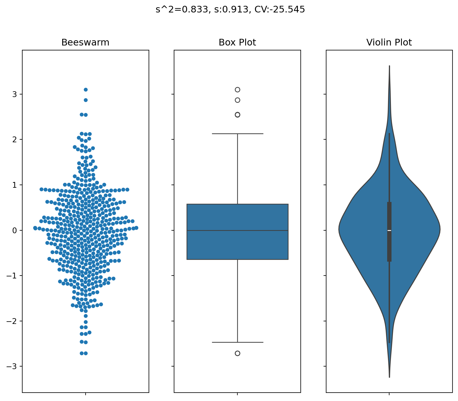
More Variable
Text(0.5, 1.0, 's^2=4.445, s:2.108, CV:2.467')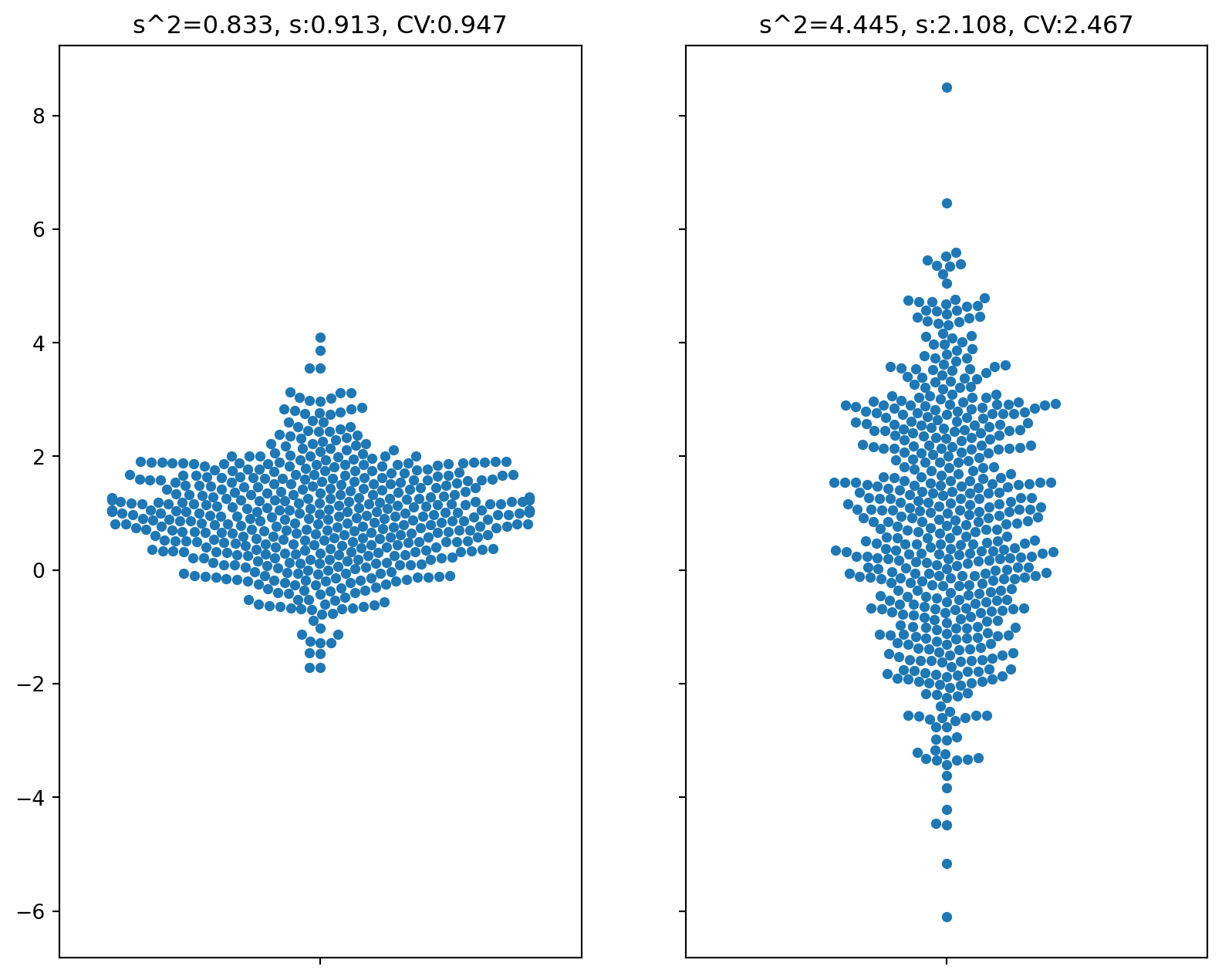
Measures of Distribution Shape, Relative Location, and Detecting Outliers
- z-Scores
- Chebyshev’s Theorem
- Empirical Rule
- Detecting Outliers
Z-scores
- The z-score is often called the standardized value.
- It denotes the number of standard deviations a data value xi is from the mean.
- An observation’s z-score is a measure of the relative location of the observation in a data set.
- A data value less than the sample mean will have a z-score less than zero.
- A data value greater than the sample mean will have a z-score greater than zero.
- A data value equal to the sample mean will have a z-score of zero.
Example

Chebyshev’s Theorem
- At least \((1 – 1/a^2)\) of the data values must be within z standard deviations of the mean, where \(a\) is any value greater than 1.
- Chebyshev’s theorem requires \(a > 1\); but \(a\) need not be an integer.
- At least 75% of the data values must be within \(a = 2\) standard deviations of the mean.
- At least 89% of the data values must be within \(a = 3\) standard deviations of the mean.
- At least 94% of the data values must be within \(a = 4\) standard deviations of the mean.
Example

Empirical Rule

Covariance and Correlation
- Finds the relationships between two variables
- The covariance and correlation measure the linear association between two variables.
- Positive values indicate a positive relationship.
- Negative values indicate a negative relationship. The covariance is computed as follows:
\[ s_{xy} = \frac{1}{N} \sum_i^N (x_i - \bar{x})(y_i - \bar{y}) \]
Correlation is:
\[ r_{xy} = \frac{s_{xy}}{s_x \cdot s_y} \]
Example

Example
