Discrete Probability Distributions
Random Variables
- A random variable is a numerical description of the outcome of an experiment.
- A discrete random variable may assume either a finite number of values or an infinite sequence of values.
- A continuous random variable may assume any numerical value in an interval or collection of intervals.
Random Variables vs. Variables
- A variable is simply a characteristic that can be measured or observed.
- A random variable is a variable whose value is determined by the outcome of a random experiment.
- If a variable is characterized by some set, say, \(\mathbb{R}+\) and nothing else, then it is just a variable.
- But a random variable is almost like a function. It is actually a map from the sample space of an experiment to a set of numbers.
- A random variable’s mapping can be described by a probability distribution.
Random Variables
| Illustration | Random Variable x | Type |
|---|---|---|
| Family size | x = Number of dependents reported on tax return | Discrete |
| Distance from home to stores on a highway | x = Distance in miles from home to the store site | Continuous |
| Own dog or cat | x = 1 if own no pet; | Discrete |
| x = 2 if own dog(s) only; | ||
| x = 3 if own cat(s) only; | ||
| x = 4 if own dog(s) and cat(s) |
Discrete Probability Distributions
- The probability distribution for a random variable describes how probabilities are distributed over the values of the random variable.
- We can describe a discrete probability distribution with a table, graph, or formula.
Discrete Probability Distributions
- The probability distribution is defined by a probability function, denoted by f(x), that provides the probability for each value of the random variable.
- The required conditions for a discrete probability function are:
\[ f(x)\geq 0 \text{ and } \sum f(x)=1 \]
What kinds of distributions are there?
- There are MANY families of distributions
- Some are mathematically interesting
- Some are based on trying to model a particular phenomenon
- Uniform
- Binomial
- Poisson
- Hypergeometric
Uniform Distribution
- Already considered this for throwing a dice
- Simplest distribution; all values of the random variable are equally likely.
- Bayesian statistics: “flat prior”
- Since every value is equally likely, I don’t really have a lot of information!
Uniform Distribution
\[ f(x) = \frac{1}{n} \]
where \(n\) is the number of value taken by x
- Notice that it is NOT a function of x!
Properties of Distributions
- Expected Value
- Variance, Covariance, Standard Deviation
Expected Value
- In econometrics, we often work with expectations of random variables
- The expectation is often denoted as \(E(X)\) for a random variable X.
- The expected value, or mean, of a random variable is a measure of its central location.
\[ E(x) = \mu = \sum x f(x) \]
- The expected value is a weighted average of the values the random variable may assume. The weights are the probabilities.
- The expected value does not have to be a value the random variable can assume.
Example
Find the expected value of a die:
| Number | f(x) | xf(x) |
|---|---|---|
| 1 | 1/6 | 1/6 |
| 2 | 1/6 | 2/6 |
| 3 | 1/6 | 3/6 |
| 4 | 1/6 | 4/6 |
| 5 | 1/6 | 5/6 |
| 6 | 1/6 | 1 |
\[ E(die) = 1/6 + 2/6 + 3/6 + 4/6 + 5/6 + 1 = 3.5 \]
The Wild World of Expectations
- For a discrete random variable, the expectation is calculated as:
\[ E(X) = \sum_i x_i P(X = x_i) \]
- For a continuous random variable, the expectation is calculated as:
\[ E(X) = \int_{-\infty}^{\infty} x f(x) dx \]
Conditional Expectation
- The conditional expectation of \(Y\) given \(X\) is defined as:
\[ E[Y|X] = \sum y p(y|X) \]
- This is the expected value of \(Y\) when we know the value of \(X\).
- Very similar to the idea of conditional probability.
The Law of Iterated Expectations
- The Law of Iterated Expectations states that:
\[ E(Y) = E(E(Y|X)) \]
- So the average of a random variable is equal to the average of its conditional averages.
Example
Given this joint probability distribution of income, show that \(E(E(Income|Female)) = E(Income)\).
| Female | Income | Joint Probability |
|---|---|---|
| 1 | 30,000 | 0.20 |
| 1 | 40,000 | 0.30 |
| 1 | 50,000 | 0.10 |
| 0 | 45,000 | 0.10 |
| 0 | 55,000 | 0.20 |
| 0 | 65,000 | 0.10 |
- First, we need to compute the marginal probabilities of Female
- Next, we compute the conditional expectations
- Finally, we compute the overall expectation and verify the law
The work: - Marginal Probabilities: - P(Female=1) = 0.20 + 0.30 + 0.10 = 0.60 - P(Female=0) = 0.10 + 0.20 + 0.10 = 0.40 - Conditional Expectations: - E(Income|Female=1) = (30,0000.20 + 40,0000.30 + 50,0000.10) / 0.60 = 38,333.33 - E(Income|Female=0) = (45,0000.10 + 55,0000.20 + 65,0000.10) / 0.40 = 55,000 - Overall Expectation: - E(E(Income|Female)) = (38,333.330.60) + (55,0000.40) = 45,000 - Now compute E(Income): - E(Income) = (30,0000.20 + 40,0000.30 + 50,0000.10 + 45,0000.10 + 55,0000.20 + 65,0000.10) = 45,000 - Thus, E(E(Income|Female)) = E(Income) = 45,000
Properties of expectations
For any constant \(a\) and random variable \(X\):
\[ E(aX) = aE(X) \]
For any random variables \(X\) and \(Y\):
\[ E(X + Y) = E(X) + E(Y) \]
The expectation operator is linear
- The expectation operator is linear, meaning that it can be distributed over sums and differences of random variables.
- How?
Suppose we have a discrete distribution with random variable X which can take on n values \(x_1, x_2, ..., x_n\) with probabilities \(p_1, p_2, ..., p_n\).
What would \(E(X)\) be?
\[ E(X) = \sum_{i=1}^{n} x_i p_i \]
Now what would \(E(aX)\) for some constant \(a\)?
\[ E(aX) = \sum_{i=1}^{n} a x_i p_i = a \sum_{i=1}^{n} x_i p_i = aE(X) \]
The expectation operator is linear
- What about \(E(X + Y)\)?
- For this we need a joint distribution of X and Y
- Let this joint distribution be \(p(x,y)\)
\[ E(X + Y) = \sum_{x} \sum_{y} (x + y) p(x,y) \]
\[ = \sum_{x} \sum_{y} x p(x,y) + \sum_{x} \sum_{y} y p(x,y) \]
\[ = \sum_{x} x \sum_{y} p(x,y) + \sum_{y} y \sum_{x} p(x,y) \]
The above step is interesting… why?
What do we do now?
What is the sum of the joint distribution (\(\sum_{y} p(x,y)\)) and analogously for \(Y\)?
\[ \sum_{y} p(x,y) = p(x, y_1) + p(x, y_2) + ... + p(x, y_n) \]
This gives us the marginal probability of \(X\). What is the marginal probability of \(Y\)?
With this we can abuse the notation a little bit…
\[ = \sum_{x} x p(x) + \sum_{y} y p(y) \]
\[ = E(X) + E(Y) \]
Variance and Covariance
- The variance summarizes the variability in the values of a random variable.
- Similar to the variance we already looked at, but using \(\mu\), not the sample mean
- Standard Deviation is the square root of the variance
- Population vs. sample
\[ Var(x) = \sigma^2 = \sum (x-\mu)^2 f(x) \]
Question: Based on this, what sign is the variance?
Example
What is the variance of a die?
| Number | x-\(\mu\) | \((x-\mu)^2\) | f(x) | \((x-\mu)^2 f(x)\) |
|---|---|---|---|---|
| 1 | -2.5 | 6.25 | 1/6 | 1.0417 |
| 2 | -1.5 | 2.25 | 1/6 | 0.375 |
| 3 | -0.5 | 0.25 | 1/6 | 0.0417 |
| 4 | 0.5 | 0.25 | 1/6 | 0.0417 |
| 5 | 1.5 | 2.25 | 1/6 | 0.375 |
| 6 | 2.5 | 6.25 | 1/6 | 1.0417 |
\[ Var(die) = 1.0417 + 0.375 + 0.0417 + 0.0417 + 0.375 + 1.0417 = 2.9167 \]
Properties of Variance
For any constant \(a\) and random variable \(X\):
\[ Var(aX) = a^2Var(X) \]
For any random variables \(X\) and \(Y\):
\[ Var(X + Y) = Var(X) + Var(Y) + 2Cov(X,Y) \]
If X and Y are independent, then \(Cov(X,Y) = 0\)
Some insight first!
When we discussed the variance, I have shown it as a sum:
\[ Var(X) = \sum_{i=1}^{n} (x_i - \mu)^2 f(x_i) \]
But if you squint your eyes, what does that sort of look like? Like an expectation!
Note
\[ Var(X) = E((X - \mu)^2) \]
The Variance of two random variables
\[ Var(X + Y) = E((X + Y - E(X + Y))^2) \]
Note
\[ Var(X + Y) = E((X + Y - E(X + Y))^2) = E((X + Y - E(X) - E(Y))^2) \]
\[ = E((X - E(X))^2 + (Y - E(Y))^2 + 2(X - E(X))(Y - E(Y))) \]
\[ = E((X - E(X))^2) + E((Y - E(Y))^2) + 2E((X - E(X))(Y - E(Y))) \]
\[ = Var(X) + Var(Y) + 2Cov(X,Y) \]
Why do we square it?
Show that \(Var(aX + b) = a^2Var(X)\)
Note
\[ Var(aX + b) = E((aX + b - E(aX + b))^2) = E((aX + b - aE(X) - b)^2) \]
\[ = E((aX - aE(X))^2) = a^2E((X - E(X))^2) = a^2Var(X) \]
Interesting, why is the \(Var(b)=0\)?
Bivariate distributions: Two die being rolled at the same time
- If a die is a uniform distribution with probability 1/6 for each event, then two die will be:
Covariance
- Covariance is:
\[ Cov(x, y) = \sigma_{xy} = \sum (x-\mu_x)(y - \mu_y) f(x,y) \]
or equivalently:
\[ Cov(X,Y) = E((X - E(X))(Y - E(Y))) \]
Properties of Covariance
For any constant \(a\) and random variable \(X\):
\[ Cov(aX, Y) = aCov(X,Y) \]
For any two constants \(a\) and \(b\):
\[ Cov(aX, bY) = abCov(X,Y) \]
For any random variables \(X\), \(Y\) and \(Z\):
\[ Cov(X + Y, Z) = Cov(X,Z) + Cov(Y,Z) \]
Review:
For any random variables \(X\) and \(Y\):
\[ Var(X + Y) = Var(X) + Var(Y) + 2Cov(X,Y) \]
Note:
- Just as with conditional expectations, conditional covariance and conditional variance are also a thing.
Independence
- If two random variables are independent, then their covariance is zero.
\[ Cov(X,Y) = 0 \]
However, the converse is not true. If the covariance of two random variables is zero, then they are not necessarily independent.
Except for a normal distribution!
Binomial Distribution
- Based on a “binomial experiment”
- The experiment consists of a sequence of n identical trials.
- Two outcomes, success and failure, are possible on each trial.
- The probability of a success, denoted by p, does not change from trial to trial.
- The trials are independent.
“How many heads will land after 25 coin flips?”
“If a machine fails after a year at a rate of 30%, what is the probability of 2 machines failing after a year?”
Constructing a Binomial for Coin Flips
- Assume a fair coin (\(p=Pr(Heads)=.5\))
- Assume each flip is independent
- Let’s just do 2 trials for now. What is the sample space?
\[ S = \{(HH), (HT), (TH), (TT)\} \]
What is the probability of each of the events?
1/2 * 1/2
What is the probability of having one Heads after two trials?
- We need to find \(Pr(Getting one Heads in two Trials)\)
- What need the number of occurrences with 1 H
- 2
\[ 2 \cdot \frac{1}{4} \]
What did we learn?
- We only need the number of occurrences where H was flipped once
What if the coin isn’t fair?
- Let’s say \(Pr(Heads) = \frac{1}{4}\)
- What would this look like now?
\[ \text{Number of occurrences of 1 H}\cdot Pr(Getting heads)\cdot Pr(Getting Tails) \]
\[ 2 \cdot \frac{1}{4} \cdot \frac{3}{4} \]
What about 3 trials?
\[ S = \{(HHH), (HHT), (HTH), (HTT), (THH), (TTH), (THT),(TTT) \} \]
What is the probability of getting one H now?
\[ 3 \cdot \frac{1}{4} \cdot \frac{3}{4} \cdot \frac{3}{4} \]
\[ 3 \cdot \frac{1}{4} \cdot (\frac{3}{4})^2 \]
Or
\[ 3 \cdot (\frac{1}{4})^{1} \cdot (\frac{3}{4})^{n-1} \]
where \(n=3\)
What did we learn?
We can write the probability expression as as a function of the number of trials and the number of “successes” we want.
Note
Solving by induction is fun!
Last Part: the Combinatorics
- The number in front of the probability expression tells us the number of times to multiply the joint probability
- This expression is really telling us the number of combinations of a given set of Heads and Tails, without the order mattering
We can write this as:
\[ C^n_x = \frac{n!}{x!(n-x)!} \]
where n is the number of trials and x is the number of successes (Heads) we want.
\[ n! = n(n-1)(n-2)...(1) \]
Note
\[ n! = n(n-1)! \]
What does that mean?
To get the intution we need to understand Combination’s counterpart, permutation
A permutation is an arrangement of objects in a definite order
So in the case of coin flips, permutations count HT, and TH as two distinct permutations, because the order of the occurrences matter.
Let’s calculate the number of permutations for coin flips for three trials.
Permutations
- There are three trial outcomes, let’s call them \(T_1\), \(T_2\) and \(T_3\).
- How many distinct ways can we arrange them?
___ ___ ___- For the first spot, we can put in either \(T_1\), \(T_2\) or \(T_3\). For the second spot, we used one of them up, so we can only use two of them. For the last spot that leads to just one trial remaining. This is just \(3!\):
\[ 3! = 3 \cdot 2 \cdot 1 \]
Generalize
If we follow the same logic, but now for \(n\) trials, we will have \(n!\) distinct ways to arrange these trails. But what if we wanted to arrange only \(r\) of them. Ex: We have 10 trials, but want to arrange into 5 spots.
___ ___ ___ ___ ___Then we would just stop when we got to \(r\).
\[ n \cdot (n-1) \cdot (n-2) \cdot ... \cdot (n-(r-1)) \]
But for mathematical niceness, we can use the properties of factorials to see that:
\[ \begin{split} & n \cdot (n-1) \cdot (n-2) \cdot ... \cdot (n-(r-1)) \\ &= \frac{n \cdot (n-1) \cdot (n-2) \cdot ... \cdot (n-(r-1))\cdot (n-r) \cdot ... \cdot (1)}{(n-r)!} \end{split} \]
And that’s a permutation!
Now combinations…
The last part is now to note that combinations don’t care about order, so HTH is the same HHT.
In the permutation then, we are counting duplicates and there are \(r!\) ways that we are double-counting them. So in that case we we just divide by \(r!\) and get the combination formula.
\[ \frac{\frac{n!}{(n-r)!}}{r!} = \frac{n!}{r!(n-r)!} \]
Back to the Bernoulli
With this knowledge, we have what we need to write out the probability distribution for the Bernoulli:
\[ f(x) = \frac{n!}{x!(n-x)!}\cdot p^x (1-p)^{(n-x)} \]
Example
Over 5 trials, what is the probability that at most 1 coins will be Heads?
Hint: Use the fact that \(Pr(Heads \leq 1) = Pr(Heads=0 \cup Heads=1)\)
Example
Evans Electronics is concerned about a low retention rate for its employees. In recent years, management has seen a turnover of 10% of the hourly employees annually.
For any hourly employee chosen at random, management estimates a probability of 0.1 that the person will not be with the company next year.
Choosing 3 hourly employees at random, what is the probability that 1 of them will leave the company this year?
\[ \begin{split} f(x) &= \frac{n!}{x!(n-x)!} p^x (1-p)^{n-x} \\ f(1) &= \frac{3!}{1!(3-1)!} (0.1)^1 (0.9)^2 = 0.243 \end{split} \]
Properties of the Bernoulli Distribution
\[ E(x) = \mu = np \]
\[ Var(x) = np(1-p) \]
Example
Using the definition of expected value, show that the expected value of a Bernoulli distribution with \(p=\frac{1}{2}\) and 2 trials is \(E(x) = np\).
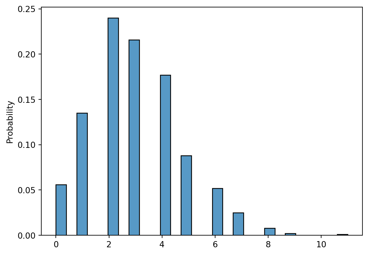
Poisson Distribution
- A Poisson distributed random variable is often useful in estimating the number of occurrences over a specified interval of time or space.
- It is a discrete random variable that may assume an infinite sequence of values (x = 0, 1, 2, . . . ).
- Examples of Poisson distributed random variables:
- number of vehicles arriving at a toll booth in one hour
- Bell Labs used the Poisson distribution to model the arrival of phone calls.
Properties of the Poisson Distribution
- The probability of an occurrence is the same for any two intervals of equal length.
- The occurrence or nonoccurrence in any interval is independent of the occurrence or nonoccurrence in any other interval.
\[ f(x) = \frac{\mu^x e^{-\mu}}{x!} \]
x = the number of occurrences in an interval \(\mu\) = the mean number of occurrences in an interval
Poisson Probability Function
- Because there is no stated upper limit for the number of occurrences, the probability function f(x) is applicable for values x = 0, 1, 2, … without limit.
- In practical applications, x will eventually become large enough so that f(x) is approximately zero and the probability of any larger values of x becomes negligible.
Properties of the Poisson Distribution
\[ \mu = \sigma^2 \]
Example
Patients arrive at the emergency room of Mercy Hospital at the average rate of 6 per hour on weekend evenings.
What is the probability of 4 arrivals in 30 minutes on a weekend evening?
\[ \frac{3^4 e^{-3}}{4!} = 0.1680 \]
Mercy Hospital
Things to keep in mind
- Discrete probability distributions have a non-zero probability at a particular event (not true for out next lecture)
- These distributions are all importand interesting, but as we’ll see most of them can be approximated with a bell curve (normal distribution) with a large enough population size.