EC031-S26
Important: Be neat or type.
Note: The problems may differ based on the edition of the textbook you have.
ASW 3.62
Solution
The mean is calculated as:
\[ \text{Mean} = \frac{\sum x_i}{n} = 2.95 \]
The median is:
\[ \text{Median} = 3 \]
The first quartile (\(Q_1\)) is:
\[ Q_1 = 1 + 0.25(1 - 1) = 1 \]
The third quartile (\(Q_3\)) is:
\[ Q_3 = 4 + 0.75(5 - 4) = 4.75 \]
The range is:
\[ \text{Range} = 7 \]
The interquartile range (IQR) is:
\[ \text{IQR} = Q_3 - Q_1 = 4.75 - 1 = 3.75 \]
The variance is:
\[ \text{Variance} = 4.37 \]
The standard deviation is:
\[ \text{Standard Deviation} = 2.09 \]
Since most people dine out a relatively few times per week, and a few families dine out frequently, the data is expected to be positively skewed. The skewness measure is:
\[ \text{Skewness} = 0.34 \]
This indicates the data is somewhat skewed to the right.
The lower limit is:
\[ \text{Lower Limit} = Q_1 - 1.5 \times \text{IQR} = -4.625 \]
The upper limit is:
\[ \text{Upper Limit} = Q_3 + 1.5 \times \text{IQR} = 10.375 \]
No values in the data are less than the lower limit or greater than the upper limit, so there are no outliers.
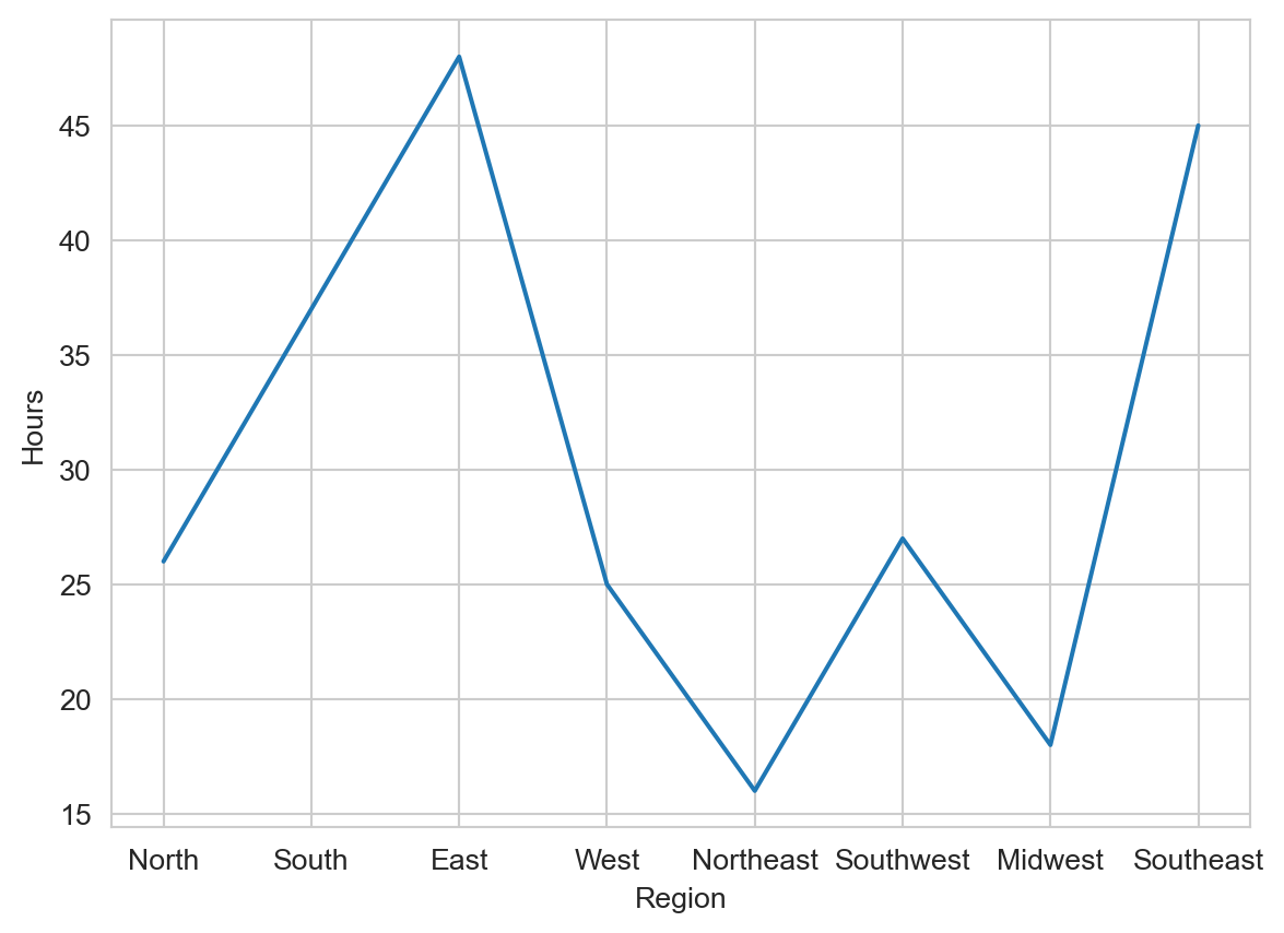
This graph shows a line graph with regions of the United States on the x-axis and the average number of hours worked per week on the y-axis (not real data). What is wrong with the way this data is visualized?
Solution
The data shows categories on the x-axis, not a continuous variable, so a line graph is not the best way to visualize it. A bar graph would be more appropriate for this data.
ASW 3.66
Solution
This is slightly higher than the mean for the study.
\[ i=\frac{p}{100}(n)=\frac{75}{100}(50)=37.5 \]
(38th position) \(Q_3=445\)
\[ \begin{aligned} & \mathrm{IQR}=445-384=61 \\ & \mathrm{LL}=Q_1-1.5 \mathrm{IQR}=384-1.5(61)=292.5 \\ & \mathrm{UL}=Q_3+1.5 \mathrm{IQR}=445+1.5(61)=536.5 \end{aligned} \]
There are no outliers.
ASW 4.55
Solution
We are given that \(P(B \mid S) > P(B)\). This means that the probability of a purchase (\(B\)) increases when the advertisement is shown (\(S\)).
Conclusion: Yes, continue the advertisement because it increases the probability of a purchase.
Assume the company’s market share is currently \(20\%\). Showing the advertisement increases the conditional probability of purchase:
\[ P(B \mid S) = 0.30 \]
Conclusion: Continuing the advertisement should increase the market share because the conditional probability \(P(B \mid S)\) is greater than the current market share.
The second advertisement shows a bigger effect than the first.
Conclusion: The company should prioritize the second advertisement if the goal is to maximize the probability of a purchase.
ASW 3.39
Solution
With \(z=2\), Chebyshev’s theorem gives:
\[ 1-\frac{1}{z^2}=1-\frac{1}{2^2}=1-\frac{1}{4}=\frac{3}{4} \]
Therefore, at least \(75 \%\) of adults sleep between 4.5 and 9.3 hours per day. b. This is from 2.5 standard deviations below the mean to 2.5 standard deviations above the mean.
With \(z=2.5\), Chebyshev’s theorem gives:
\[ 1-\frac{1}{z^2}=1-\frac{1}{2.5^2}=1-\frac{1}{6.25}=.84 \]
Therefore, at least \(84 \%\) of adults sleep between 3.9 and 9.9 hours per day. c. With \(z=2\), the empirical rule suggests that \(95 \%\) of adults sleep between 4.5 and 9.3 hours per day. The percentage obtained using the empirical rule is greater than the percentage obtained using Chebyshev’s theorem.
ASW 4.48
Solution
\(0.5029\)
\(0.5758\)
No, from part a we have \(P(F) = 0.5029\), and from part b we have \(P(A|F) = 0.5758\). Because \(P(F) \neq P(A|F)\), events A and F are not independent
Important
Make sure to submit the do-file along with the rest of your problem set.
STATA Exercise. This should be a reasonable follow-up to your Intro to STATA workshop. The dataset that you downloaded contains the Employee Attrition Prediction Dataset, representing a variety of employees from different departments and roles within an organization. It includes demographic information, job-related metrics, performance evaluations, and factors that influence employee attrition (turnover). The dataset is designed for use in analysis of employee retention.
Helpful note: You can access STATA’s help by typing help (without the quotes), where what goes in the blank is the command you are trying to execute. For example, in part (a), you’d type help import delimited in the command window (again, without the quotes).
Instructions:
In Stata, open the Do File Editor (in Window menu), and in that editor, open the Stata executable file, ps1.do. You will modify this .do file to perform the tasks below. Copy-paste or take screenshots of the relevant output and include it in your problem set when you submit.
summarize command to display means, standard deviations, minima, and maxima, for all variables in this data set. To do this for only some variables, type summarize var1 var2.... What kind of data are these (e.g. cross-sectional, time series, or longitudinal, etc)? Explain how you know.job_level, monthly_income and age. What kind of variable is each of these? Are they continuous or discrete? Are they ordinal or nominal?histogram to create a histogram of age. You do not need to submit this graph, but please describe the shape of the distribution. Is it symmetric? Bell-shaped? Skewed right or left?generate command to generate a variable called weekly_rate, which is the hourly rate of pay multiplied by 40 hours per week.scatter to create a scatter plot with age on the x-axis and weekly_rate on the y-axis. Screenshot/save this graph to submit with your problem set.correl command to calculate the correlation coefficient for these two variables. Does the sign of the correlation coefficient make sense to you? What about its magnitude?Solution
The data here is cross-sectional. This is because the data is collected at a single point in time, and the variables are not repeated over time. There are 1000 employees and 1000 observations in the dataset.
job_level: This is a discrete variable. It is ordinal because it represents the level of the job, which is ranked from 1 to 5. monthly_income: This is a continuous variable. It is ordinal because it represents the monthly income of the employee. age: This is a continuous variable. It is ordinal because it represents the age of the employee.
The correlation coefficient is positive, which makes sense because as age increases, the weekly rate is also likely to increase. But the magnitude of the correlation coefficient indicates a very small positive relationship between age and weekly rate.