Group Outlines Due
- Project Outlines due April 3rd
- Structure:
- Introduction and Motivation
- Data
- How easily available is it?
- Did you decide to use an alternative dataset?
- Methods
- What does the paper use?
- How available is replication code?
- Describe what the method is doing
- Additions/Extensions
Agenda
- Sampling Distribution of \(b_1\)
- Confidence Intervals in Regression
- Hypothesis Testing in Regression
- Residual Analysis
- Validating Assumptions
- Outliers and Influential Variables
Review
\[
b_1 = \frac{\sum_{i=1}^n (x_i - \bar{x})(y_i - \bar{y})}{\sum_{i=1}^n (x_i - \bar{x})^2}
\]
- If we can show that \(b_1\) is normally distributed
- Then we can standardize \(b_1\) for use in confidence intervals and hypothesis tests as long as we know its expectation and variance.
The Mean and Variance of \(b_1\)
- We know from previous lectures that
\[
E(b_1) = \beta_1
\]
- Now what is the variance of the estimator?
\[
Var(b_1) = \frac{\sigma^2_{\varepsilon}}{\sum_{i=1}^n (x_i - \bar{x})^2}
\]
Unknown \(\sigma^2_{\varepsilon}\)
- Once again, since we don’t know \(\sigma^2_{\varepsilon}\)
- Once again we use the sample analog
- For this we can use
\[
s^2 = \frac{\sum_{i=1}^n (y_i - \hat{y}_i)^2}{n-2}
\]
So the standard error of \(b_1\) is:
\[
s_{b_1} = \sqrt{\frac{\frac{\sum_{i=1}^n (y_i - \hat{y}_i)^2}{n-2}}{\sum_{i=1}^n (x_i - \bar{x})^2}}
\]
How is \(b_1\) Distributed?
\[
b_0 = \bar{y} - b_1\bar{x}
\]
\[
b_1 = \frac{\sum_{i=1}^n (x_i - \bar{x})y_i}{\sum_{i=1}^n (x_i - \bar{x})^2}
\]
- … and expand \(y_i\) using the population model (remember the trick about centering \(y_i\)):
\[
= \frac{\sum_{i=1}^n (x_i - \bar{x})(\beta_0 + \beta_1x_i + \varepsilon_i)}{\sum_{i=1}^n (x_i - \bar{x})^2}
\]
\[
= \beta_1 + \frac{\sum_{i=1}^n (x_i - \bar{x})\varepsilon_i}{\sum_{i=1}^n (x_i - \bar{x})^2}
\]
Distribution of \(b_1\)
\[
\varepsilon_i | x_i \sim N(0, \sigma^2_{\varepsilon})
\]
- If we assume that \(x_i\) are fixed, then A5 is really just:
\[
\varepsilon_i \sim N(0, \sigma^2_{\varepsilon})
\]
- Then \(b_1\) is a linear combination of normally distributed random variables, and thus is also normally distributed.
\[
b_1 \sim N\left(\beta_1, \frac{\sigma^2_{\varepsilon}}{\sum_{i=1}^n (x_i - \bar{x})^2}\right)
\]
Confidence Intervals
Then the \(1-\alpha\) confidence interval for \(b_1\) is:
\[
b_1 \pm t_{\alpha/2, n-2}s_{b_1}
\]
And the two-sided hypothesis test is then:
\[
H_0: \beta_1 = 0 \quad \text{vs.} \quad H_1: \beta_1 \neq 0
\]
We reject if:
\[
|\frac{b_1 - \beta_1}{s_{b_1}}| > t_{\alpha/2, n-2}s_{b_1}
\]
Interpreting Coefficients
- The coefficient \(b_1\) is the expected change in \(y\) for a one unit change in \(x\).
\[
b_1 = \frac{\Delta y}{\Delta x}
\]
- Depending on \(y\) and \(x\) this will have different interpretations.
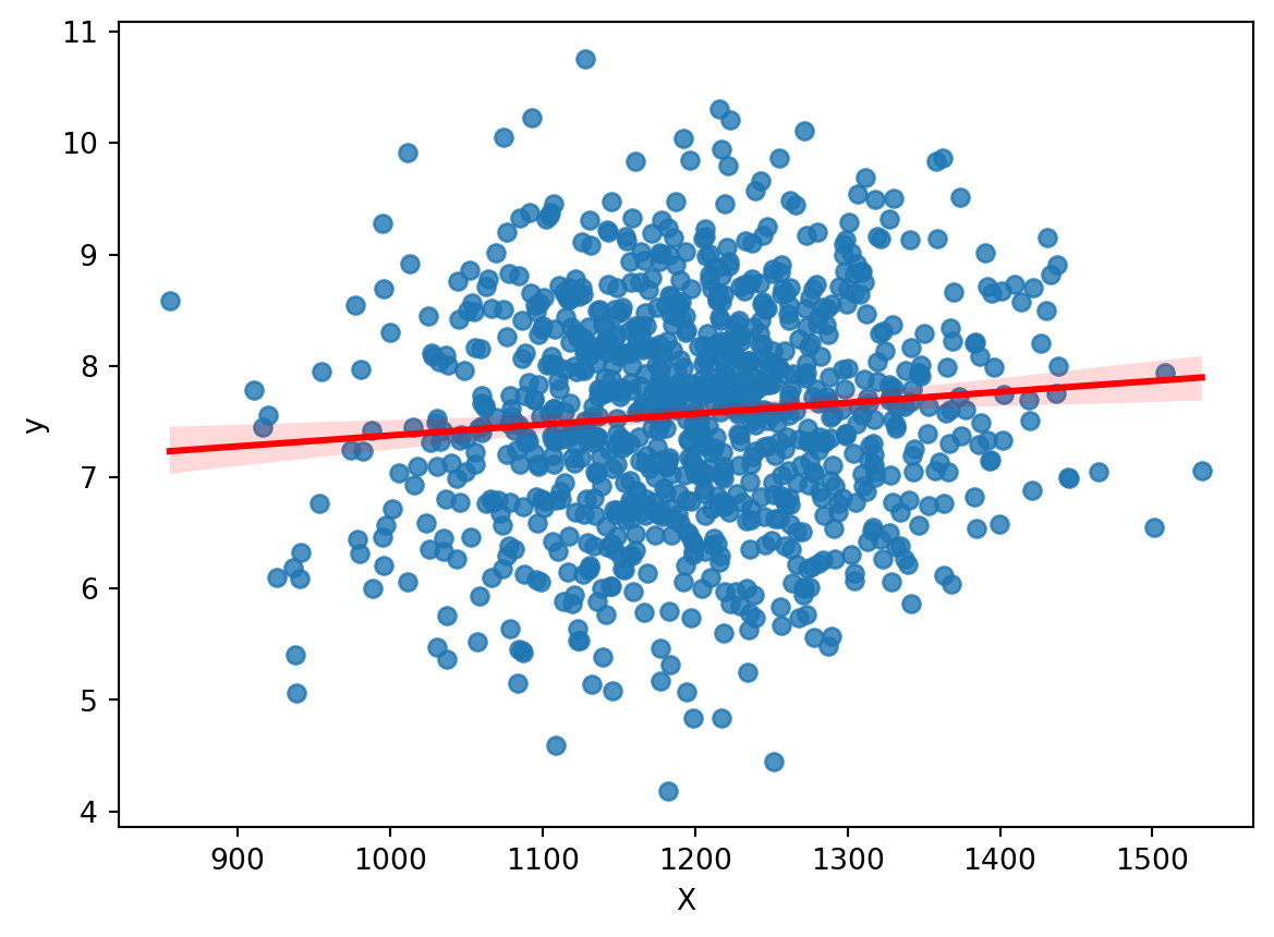
Example
.
. regress y X

      Source |       SS           df       MS      Number of obs   =     1,000
-------------+----------------------------------   F(1, 998)       =      9.38
       Model |  9.27810127         1  9.27810127   Prob > F        =    0.0022
    Residual |   986.85677       998  .988834439   R-squared       =    0.0093
-------------+----------------------------------   Adj R-squared   =    0.0083
       Total |  996.134871       999  .997132003   Root MSE        =     .9944

------------------------------------------------------------------------------
           y | Coefficient  Std. err.      t    P>|t|     [95% conf. interval]
-------------+----------------------------------------------------------------
           X |   .0009776   .0003192     3.06   0.002     .0003513    .0016039
       _cons |   6.397407   .3834314    16.68   0.000     5.644982    7.149831
------------------------------------------------------------------------------

.
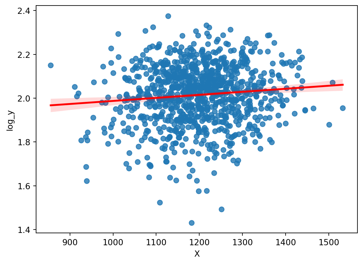
Example
.
. gen log_y = log(y)

. regress log_y X

      Source |       SS           df       MS      Number of obs   =     1,000
-------------+----------------------------------   F(1, 998)       =     10.22
       Model |  .186858023         1  .186858023   Prob > F        =    0.0014
    Residual |  18.2403713       998  .018276925   R-squared       =    0.0101
-------------+----------------------------------   Adj R-squared   =    0.0091
       Total |  18.4272293       999  .018445675   Root MSE        =    .13519

------------------------------------------------------------------------------
       log_y | Coefficient  Std. err.      t    P>|t|     [95% conf. interval]
-------------+----------------------------------------------------------------
           X |   .0001387   .0000434     3.20   0.001     .0000536    .0002239
       _cons |   1.848797   .0521288    35.47   0.000     1.746503    1.951092
------------------------------------------------------------------------------

.
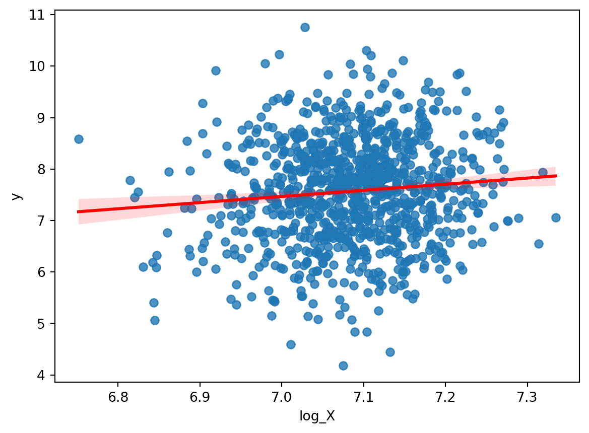
Example
.
. gen log_X = log(X)

. regress y log_X

      Source |       SS           df       MS      Number of obs   =     1,000
-------------+----------------------------------   F(1, 998)       =      9.89
       Model |  9.77239463         1  9.77239463   Prob > F        =    0.0017
    Residual |  986.362477       998  .988339155   R-squared       =    0.0098
-------------+----------------------------------   Adj R-squared   =    0.0088
       Total |  996.134871       999  .997132003   Root MSE        =    .99415

------------------------------------------------------------------------------
           y | Coefficient  Std. err.      t    P>|t|     [95% conf. interval]
-------------+----------------------------------------------------------------
       log_X |    1.19116   .3788109     3.14   0.002     .4478024    1.934517
       _cons |  -.8707322   2.683844    -0.32   0.746    -6.137357    4.395893
------------------------------------------------------------------------------

.
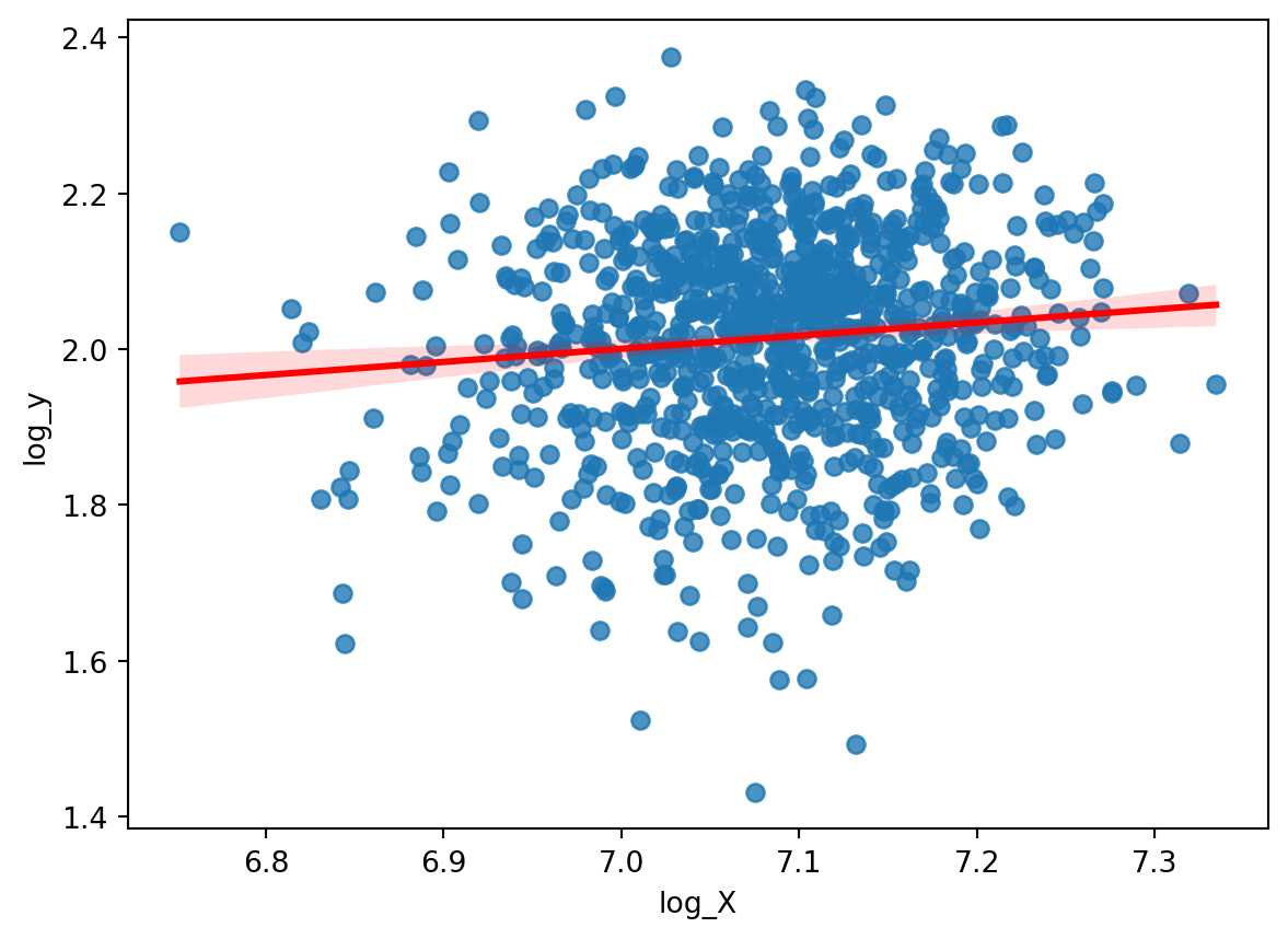
Example
.
. regress log_y log_X

      Source |       SS           df       MS      Number of obs   =     1,000
-------------+----------------------------------   F(1, 998)       =     10.74
       Model |   .19621207         1   .19621207   Prob > F        =    0.0011
    Residual |  18.2310173       998  .018267552   R-squared       =    0.0106
-------------+----------------------------------   Adj R-squared   =    0.0097
       Total |  18.4272293       999  .018445675   Root MSE        =    .13516

------------------------------------------------------------------------------
       log_y | Coefficient  Std. err.      t    P>|t|     [95% conf. interval]
-------------+----------------------------------------------------------------
       log_X |   .1687844   .0515003     3.28   0.001     .0677231    .2698457
       _cons |   .8191735   .3648753     2.25   0.025     .1031627    1.535184
------------------------------------------------------------------------------

.
Binary Variables as Independent Variables
- In some cases, \(X\) is a categorical variable.
- So 1 if male, or 0 if female
- 1 if treated, 0 if control
- 1 if college educated, 0 if not
- etc…
- What is the interpretation of \(b_1\) in this case?
\[
y = \beta_0 + \beta_1 Female + \varepsilon
\]
Interpretation
- Let’s take expectations to find out:
\[
E(y|Female=1) = \beta_0 + \beta_1
\]
\[
E(y|Female=0) = \beta_0
\]
So \(\beta_1\) is:
\[
\beta_1 = E(y|Female=1) - E(y|Female=0)
\]
- What is the interpretation of \(\beta_0\)?
Encoding Categorical/Binary Variables
- Sometimes, we can also encode a continuous variable as a categorical variable.
- Say you want to look at the effect of drought on health outcomes.
- Usually, drought is measured as a continuous variable
- Many different ways to measure drought severity that includes variables on rainfall, temperature, vegetation indices, etc…
- Let’s take a drought index that only incorporates rainfall
- The SPI
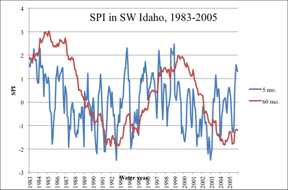
The SPI
- The Standardized Precipitation Index (SPI) is a commonly used index to measure drought severity.
- The SPI is calculated by fitting a probability distribution to historical precipitation data for a location, and then transforming the data to a standard normal distribution.
- The SPI can be calculated for different time scales, such as 1 month, 3 months, 6 months, etc…
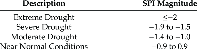
- The SPI values can then be categorized into different drought severity levels.
Using Categorical/Binary Variables in Regression
- The SPI ranges from approximately -3 to +3.
![]()
- Let’s say you want to understand the effect of drought severity on malnutrition.
- What would using the SPI directly look like?
\[
MN_i = \beta_0 + \beta_1 SPI_i + \varepsilon_i
\]
- What would the interpretation of \(\beta_1\) be?
- Does this tell you anything about drought?
Using Categorical/Binary Variables in Regression
- Instead, you can create categorical variables for drought severity.
- You can say that if SPI < -2, then extreme drought
- So generate a variable that is 1 if extreme drought, 0 otherwise.
| -2.5 |
1 |
| 1 |
0 |
| -1 |
0 |
| 1.2 |
0 |
| 3 |
0 |
\[
MN_i = \beta_0 + \beta_1 Drought_i + \varepsilon_i
\]
Now what is the interpretation of \(\beta_1\)?
\[
\beta_1 = E(MN|Drought=1) - E(MN|Drought=0)
\]
Binary Variables as the Dependent Variable
- What if the dependent variable is binary?
- 1 if employed, 0 if not
- 1 if college educated, 0 if not
- 1 if voted, 0 if not
- Can we still use linear regression?
- Yes, but it would now be called a Linear Probability Model (LPM).
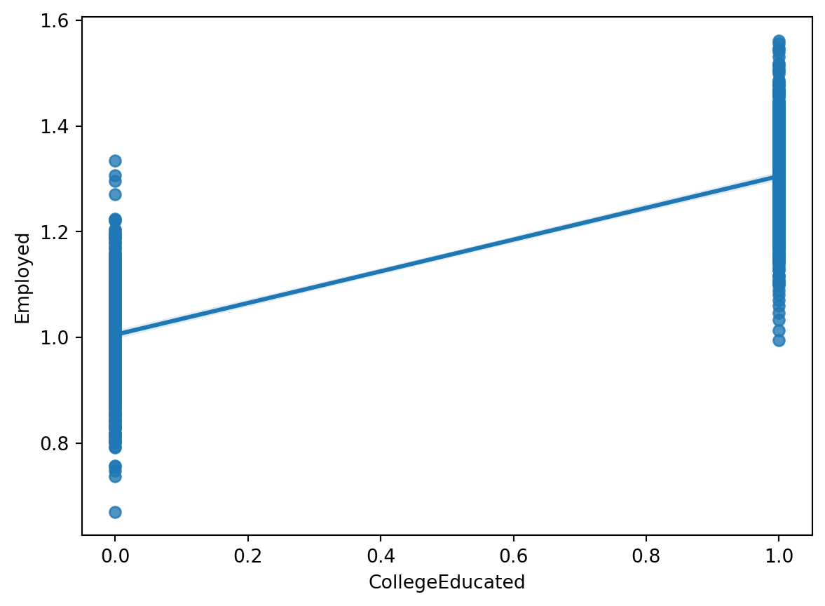
Binary Dependent Variable
- Let’s say you wanted to model employment status:
\[
Employed_i = \beta_0 + \beta_1 CollegeEducated_i + \varepsilon_i
\]
What’s the conditional expectation function of this model?
\[
E(Employed|CollegeEducated) = \beta_0 + \beta_1 CollegeEducated
\]
- Since Employed is binary, what does \(E(Employed|CollegeEducated)\) represent?
- An easy way to see this is by using the
\[
E(Employed|CollegeEducated) = \sum_{j=0}^1 P(Employed=j|CollegeEducated) \cdot j
\]
\[
= P(Employed=1|CollegeEducated) \cdot 1 + P(Employed=0|CollegeEducated) \cdot 0
\]
\[
= P(Employed=1|CollegeEducated)
\]
- So the conditional expectation function is the probability of being employed given college education.
- So the interpretation of \(\beta_1\) is:
- A one unit increase in CollegeEducated (i.e. going from not college educated to college educated) is associated with a \(\beta_1\) increase in the probability of being employed.
Residual Analysis
- Once a regression is run, we have a new object we can look at, \(\hat{y}\), the prediction.
- The residuals are the difference between the actual value, \(y\) and the prediction, \(\hat{y}\).
- The residuals provide all the information not capture by the model and is a measure of \(\varepsilon\).
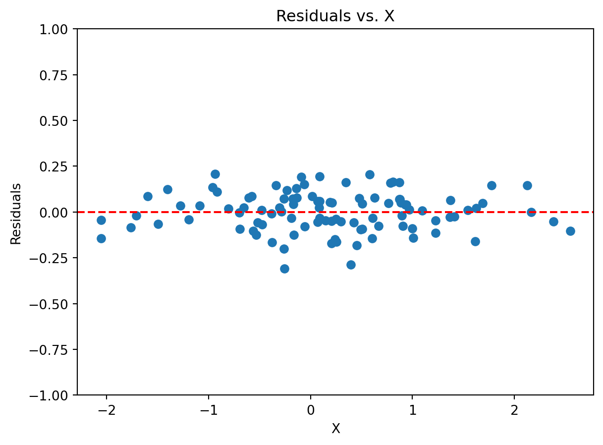
Residual Analysis
- Often a good way to work with the residuals is to graph them.
- This gives us a way to visually inspect the residuals and whether our assumptions hold.
- What do we know about what the residuals sum to?
Text(0.5, 1.0, 'Residuals vs. X')
Residual Analysis
- Recall A3: Homoskedasticity
\[
\text{Var}(\varepsilon_i|X) = \sigma^2_{\varepsilon}
\]
- This means that once we condition on \(X\), the variance of the residuals is constant.
- If we see that the residuals are around the 0 line, then we can say that we have a good fit for the linear model
- If the residuals are around the same amount apart from the 0 line, then we can say that we have homoskedasticity.
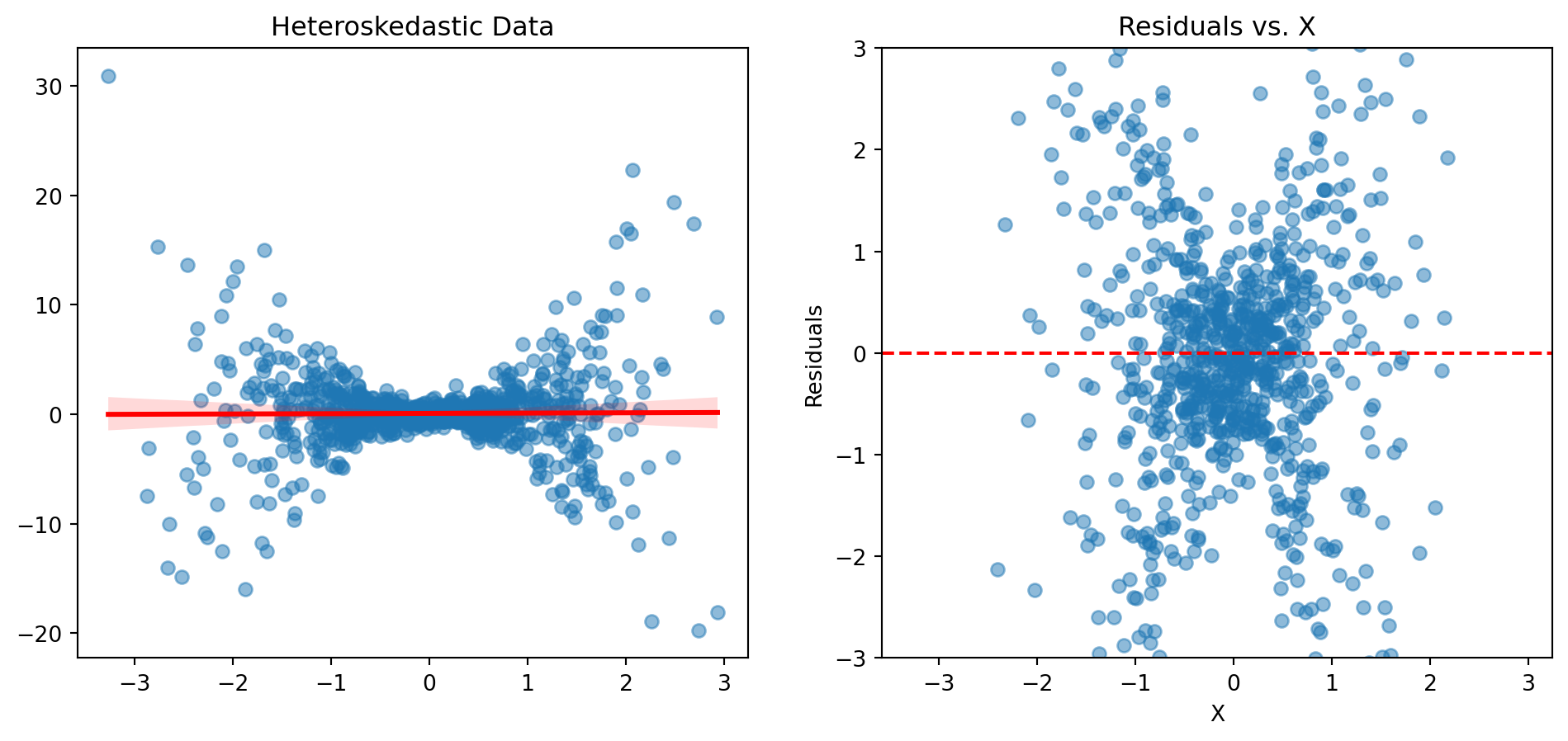
Heteroskedasticity
- What if A3 is violated?
- Then we have heteroskedasticity.
Text(0.5, 1.0, 'Residuals vs. X')
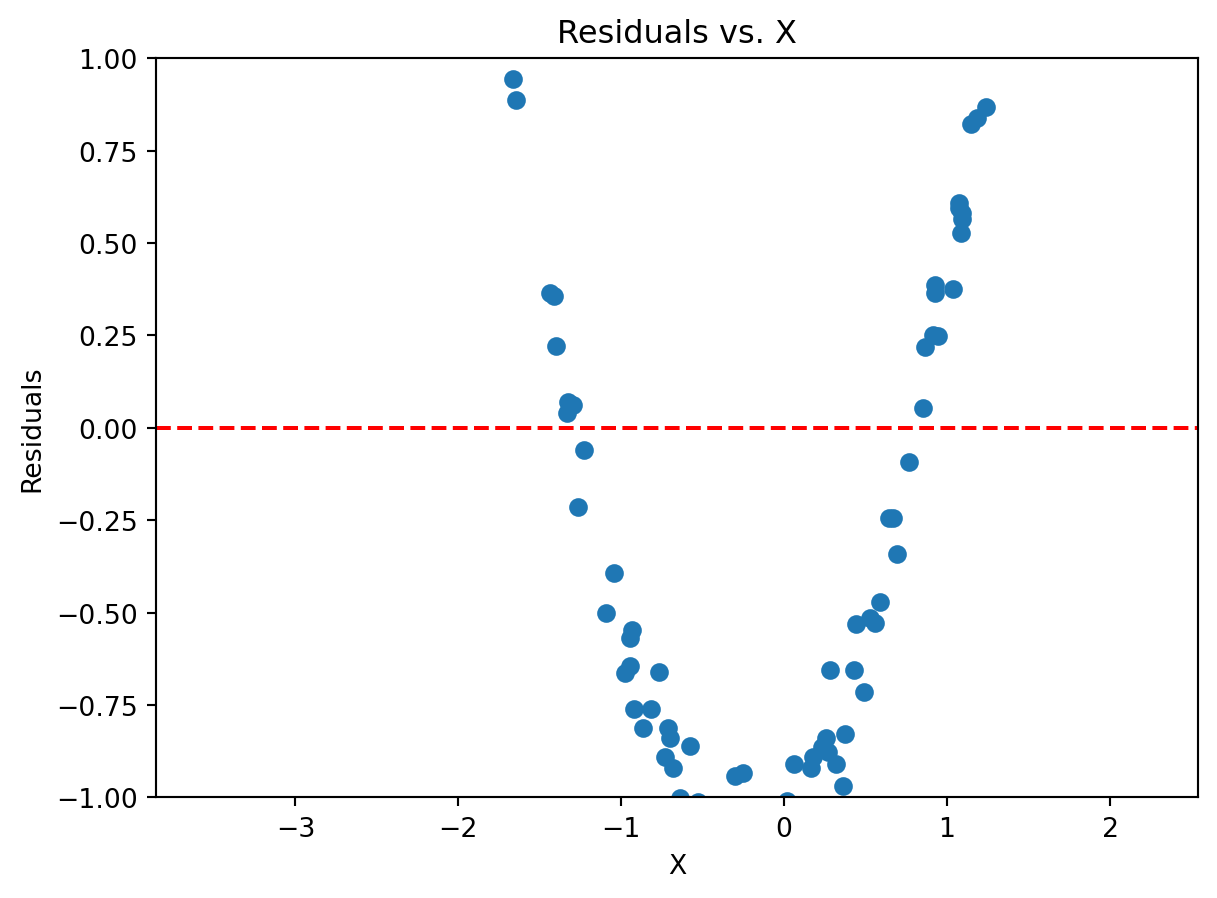
Inadequate Model
- If the residuals are not around the 0 line, then we can say that the model is inadequate.
- For instance, if a variable has some non-linear relationship with the dependent variable, then the residuals will not be around the 0 line.
Suppose we have a population model:
\[
y = \beta_0 + \beta_1 X^2 + \varepsilon
\]
But we don’t know that X has a squared term… If we run a linear regression like so:
\[
y = \beta_0 + \beta_1X + \varepsilon
\]
The squared relationships will be in the residuals.
Text(0.5, 1.0, 'Residuals vs. X')