Group Project Sign-up on front page of website and on Moodle.
Please sign up for a group by the end of the week.
There are spots starting from next Monday
If none of these times work for you, please let me know BEFORE Friday
Group Project Requirements
15 minute presentation
Either in-person or pre-recorded
Pre-recorded doesn’t necessarily have to be a presentation format, just anything that conveys the information
And we will watch it together in class
5 minutes Q&A
If you pre-record, you still need to be present for the Q&A
Group Project Grading
Presentation needs to convey:
How well you replicate the results (as a function of how easily replicable the paper was)
If you choose a paper that was easy to replicate, then you need to make sure that everything replicates perfectly. But oftentimes, this is not the case. So if the replication package was difficult to implement for whatever reason (difficult to understand code, missing data, missing output), you should highlight this in your presentation, and explain why replication wasn’t possible.
A breakdown of issues you faced, how you overcame them or what you did to get as close as possible to replication
Any extensions to the original paper
Replicating is hard enough, but the true test of a researcher is to push beyond that and think of an interesting extension. This need not be a completely new and innovative idea. It might just be using the data and exploring the data more (running a regression with a new interaction that the original paper didn’t)
Topics and thoughts about future research
Did you end up still being interested in this paper?
Would you want to continue on this line of research?
What are some questions you would want to explore in future research?
Group Project Deliverables
Submit a Replication Package of your replication
A zip file with all relevant do-files and extensions you made that can be replicated by me.
Professor Wang’s workshop will go through a replication package, best practices and how to do this.
Agenda
What is omitted variable bias (review)?
Why is it a threat to causal inference?
How to deal with omitted variable bias?
Proxy variables
Instrumental variables
What is omitted variable bias?
Omitted variable bias is a type of bias that occurs when a model does not include one or more relevant variables.
This can lead to biased estimates of the causal effect of the included variables on the outcome variable.
If our true model is:
\[
Y = \beta_0 + \beta_1 D + \beta_2 X + \varepsilon
\]
But suppose you run a “naive” regression:
\[
Y = \tilde{\beta}_0 + \tilde{\beta}_1 D + \tilde{\varepsilon}
\]
Then \(\tilde{\varepsilon} = \beta_2 X + \epsilon\).
The Oregon Health Insurance Experiment is one of the most well known natural experiments in public health. - It is the first study to use a randomized design to examine the impact of access to Medicaid. - It was not designed to be an RCT, but it turned out very RCT-like. - “[i]n early 2008, Oregon opened a waiting list for its Medicaid program for low-income adults that had previously been closed to new enrollment. Approximately 90,000 people signed up for the available 10,000 openings. The state drew names from this waiting list by lottery to fill the openings.”
- You can call this a “pipeline” randomization. - Randomness came from who got it and who didn’t
The independence assumption is then:
\[
Y_{withMedicaid} , Y_{withoutMedicaid} \perp \text{Receiving Medicaid from Oregon}
\]
The Oregon Health Insurance Experiment
What would happen if this wasn’t a lottery, but that it was “first-come, first-served”?
Could we still argue that the independence assumption holds?
What would happen to the treatment effect? How would sample selection bias change it?
The Oregon Health Insurance Experiment
By comparing the outcomes of 29,589 people who eventually received access through the lottery against 28,816 people who applied but did not win, the researchers involved have published several papers. - The results of the first two years, reviewed here, were that access to Medicaid:
increased the use of health-care services: more hospitalizations, emergency-department visits, outpatient visits, prescription-drug use, and preventive-care use.
decreased financial strain: fewer medical debts, lower likelihood of borrowing money or skipping other bill payments to cover medical expenses, and a virtual elimination catastrophic out-of pocket medical expenditures.
improved self-reported health and reduced rates of depression, but had no statistically significant effect on physical health outcomes.
had no statistically significant effect on employment or earnings.
Example: Lifetime Earnings and the Vietnam Era Draft Lottery
Josh Angrist’s PhD thesis examined whether serving in the army negatively affected people’s future income.
This is trickier to estimate than it may seem.
Simply comparing the wages of people who served in the army against those who didn’t would not be evidence of a causal relationship.
Why?
Example: Lifetime Earnings and the Vietnam Era Draft Lottery
Since people who enter the army may differ in important ways from those who don’t, and these differences may in turn affect their income potential.
In other words, the independence assumption we want is:
What would be the sign of the selection bias? - Why?
Example: Lifetime Earnings and the Vietnam Era Draft Lottery
What is really needed is a source of randomization which takes a group of men and forces some of them into the army.
A randomization tool was provided in the 1970s by the American government, which ran televised draft lotteries during the Vietnam War to select young men to be inducted into the army.
This process essentially placed otherwise similar men into a treatment and control group randomly based on selecting birth days of the year ranging from 1 to 366 (February 29 was included).
By combining the birth records of those born in 1950-53 with later earnings data drawn from a 1% sample of all social security numbers, Angrist found that, among white men, drafted veterans went on to earn 15% less than their peers who had avoided the army.
Example: Minimum Wages and Employment
David Card & Alan Krueger’s research design was simple.
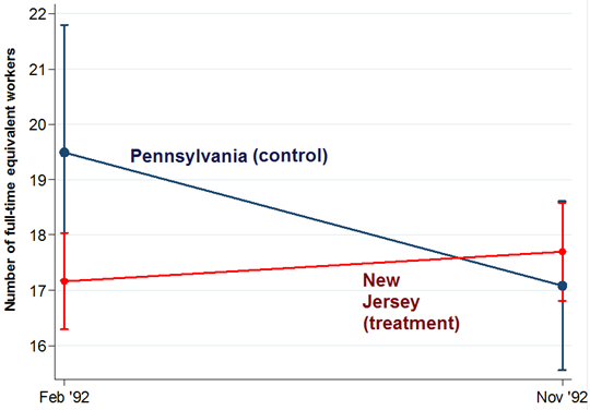
To quote their abstract: “On April 1, 1992, New Jersey’s minimum wage rose from $4.25 to $5.05 per hour. To evaluate the impact of the law we surveyed 410 fast-food restaurants in New Jersey and [neighbouring] eastern Pennsylvania before and after the rise. Comparisons of employment growth at stores in New Jersey and Pennsylvania (where the minimum wage was constant) provide simple estimates of the effect of the higher minimum wage”.
Example: Minimum Wages and Employment
Since Pennsylvania did not change its minimum wage, this makes it the control group.
If we consider New Jersey and Pennsylvania to be comparable, then we would have expected to see Pennsylvania’s downward sloping trend replicated in New Jersey if New Jersey had not increased its minimum wage.
But we don’t see this; in fact there is a slight increase in the average number of employees in New Jersey restaurants.
The authors interpret this as showing that the rise in the minimum wage did not reduce employment.
This is what will later be known as difference-in-difference estimation.
Example: Minimum Wages and Employment
Although this natural experiment does not strictly pass the independence assumption:
Difference in difference designs recover the causal effects by assuming that even if there is selection into treatment (i.e. New Jersey changing its minimum wage is probably not random), the change in the outcome variable (i.e. employment) would have been the same in both groups if the treatment had not occurred.
This is called the parallel trends assumption.
Example: The Impact of the Mariel Boatlift on the Miami Labor Market
A majority of economists agree that the average American citizen would be better off if more low-skilled and high-skilled immigrants were allowed to enter the US each year
One frequently raised concern, aside from issues of social cohesion, is that the arrival of immigrants might negatively disrupt the economy and make it more difficult for local workers to secure good jobs.
Example: The Impact of the Mariel Boatlift on the Miami Labor Market
David Card examined this issue by looking at the labor market effects of the “Mariel boatlift”, the name given to the arrival of 125,000 Cubans into Florida during April - September 1980.
This sudden arrival of relatively unskilled young men increased the size of the Miami labor force by 7%.
So once again another example of a shock that that happened so suddenly that it is hard to imagine that people could have reacted to it in any way.
Example: The Impact of the Mariel Boatlift on the Miami Labor Market
By comparing Miami with other cities which were not affected by the Mariel boatlift, Card showed that the arrival of the Mariel workers did not notably affect the wages and employment rates of the existing unskilled workers living in Miami.
Card’s approach was similar to something called “synthetic control”
Example: The Impact of the Mariel Boatlift on the Miami Labor Market
Two similar studies examined the labor market effects of the arrival of 900,000 French Algerians into France when Algeria declared independence in 1962 (Hunt, 1992), - 600,000 Russians into Israel over 1989-95 as the Soviet Union collapsed (Friedberg, 2001) - Like the Mariel study, neither of these studies found harmful effects of immigration on local labor markets. - The results of these studies, and an enormous amount of comments citing objections to the generalizability of their conclusions, are further discussed in this a New York Times article from 2015.
Using Maimonides’ Rule to Estimate the Effect of Class Size on Scholastic Achievement
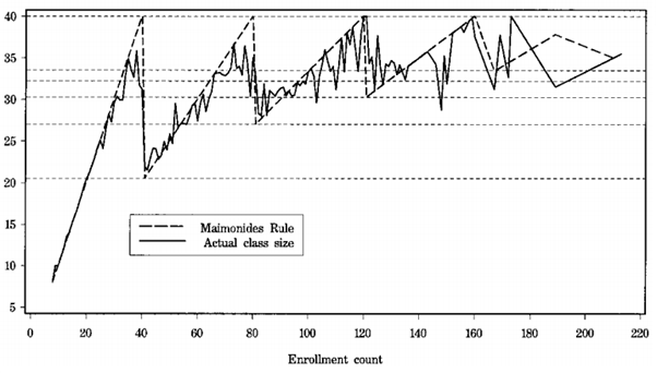
Angrist & Levy exploited an 800 year old rule governing the size of Israeli classrooms to examine whether smaller classes improved student performance.
The rule is derived from the teachings of the 12th century scholar Maimonides who said:
Twenty-five children may be put in charge of one teacher. If the number in the class exceeds twenty-five but is not more than forty, he should have an assistant to help with the instruction. If there are more than forty, two teachers must be appointed
So a strict application of this rule would mean that if 80 students were enrolled in a school, they should placed in two classes of 40 pupils each. If 81 students were enrolled, they should be placed in three classes of 27 pupils each.
This rule generated sharp discontinuities in class sizes in the schools examined by the authors, as shown in the graph.
They found that reductions in class size improved maths and reading scores for fifth graders, improved reading scores for fourth graders and had no effect on third graders.
Example: Relationships Between Poverty and Psychopathology
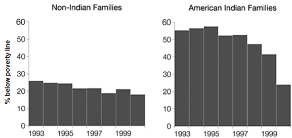
This article examined the relationship between poverty and childhood mental health. Specifically, the authors used data from the North Carolina based Great Smoky Mountains Study to test whether the environmental stresses associated with poverty caused poor mental health in children.
Over 1993-2000 this study conducted annual mental health assessments of 1420 rural children, 350 of whom were American Indian.
Over the 8 years of the study, children living below the federal poverty line were 60% more likely to have a psychiatric disorder.
Example: Relationships Between Poverty and Psychopathology
In 1996, a casino opened on the local Indian reservation and began paying the American Indians in the study a percentage of the profits every 6 months. - This payment increased each year and had reached $6000 by 2001. - Children’s earnings were paid into a trust fund until they were aged 18. - This cash injection reduced the poverty rate of Indian families while non-Indian families remained relatively unaffected
Example: Relationships Between Poverty and Psychopathology
By tracking the Indian families who moved out of poverty as a result of this income boost, the authors found that these children had a large decrease in behavioral problems, although there was no effect on the rate of depression or anxiety problems.
Improved parental supervision explained over three quarters of the effect of decreased poverty on the number of child psychiatric symptoms in the years after the casino opened,
Additional analysis suggested that this was due to a reduction in time constraints within the family; e.g. in the families that moved out of poverty, the number of single-parent households decreased and the number of households with 2 working parents increased.
Example: The Colonial Origins of Comparative Development
Does a country need good institutions (e.g. market economy, strong property rights, independent judiciary, checks and balances on government power) in order to promote economic growth, or does economic growth lead to strong institutions?
This is not just an idle historical question – a strong answer either way would have implications today for how institutions like the IMF work with developing countries.
Acemoglu et al. examined this in their very famous 2001 paper by comparing the outcomes of colonized countries.
Example: The Colonial Origins of Comparative Development
Their argument runs as follows:
There was considerable variation in colonization policies among nations colonized by Europeans. This variation led to different kinds of institutions being created in the colonized states.
At one end of the spectrum were purely extractive states such as the Belgian Congo which did not promote private property or limit government expropriation, at the other end were states such as Australia and the United States which received many European immigrants and tried to replicate European institutions.
The different colonization strategies were influenced by the feasibility of settlements.
In areas with high rates of disease and mortality among the European settlers, they were more likely to set up extractive institutions since they could not settle there in the long-term.
The kind of institutions set up by the European colonists persisted for many years afterwards, even after the countries became independent.
Example: The Colonial Origins of Comparative Development
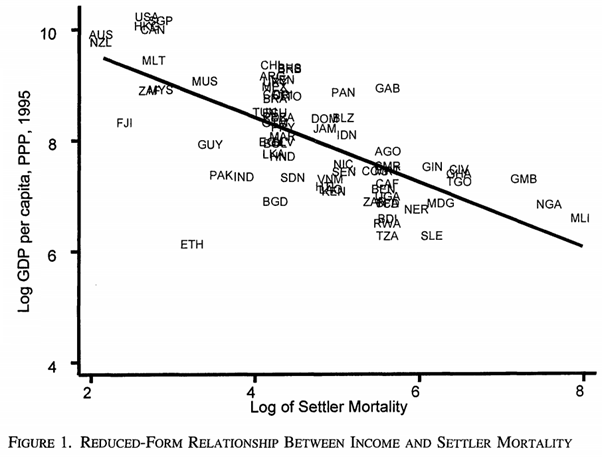
The authors created a measure of #2 by drawing on historical data on the mortality rates of sailors, bishops and soldiers in the colonies during the 1600-1800s.
The figure shows the log of these settler mortality rates against the log of GDP per capita in 1995 for some of the 75 countries the authors examined. The trend is clear; colonies in which Europeans died at a higher rate (e.g. Gambia, Mali, Nigeria) are much poorer than colonies which provided safer environments (e.g. Australia, Canada, Fiji).
This trend also holds when excluding Africa and the relative outliers of Australia, Canada, New Zealand and the US.
The authors interpret this as evidence that good institutions causally improve economic growth.
Example: The Colonial Origins of Comparative Development
This independence assumption is trickier.
The authors argue that the mortality rates of sailors, bishops and soldiers in the colonies during the 1600-1800s are exogenous to the economic growth of the countries.
But this is a bit of a stretch.
Essentially, the independence assumption is:
\[
E\big[GDPToday^{GoodInst}\mid GoodInst\big], E\big[GDPToday^{BadInst}\mid BadInst\big] \perp \text{Quality of Institutions}
\]
This is most DEFINITELY VIOLATED
So Acemoglu et al. try to argue that there’s SOMETHING else going on that is correlated with the quality of institutions, and that is ONLY correlated with GDP through the quality of institutions.
This is where a DAG would be helpful…
graph LR;
    A[Settler Mortality] --> B[Democratic Institutions]
    B --> C[GDP Today]
    B --> U[Unobserved Factors]
    U --> C
Conditional on the controls included in the regression, the mortality rates of European settlers more than 100 years ago have no effect on GDP per capita today, other than their effect through institutional development.
Instrumental Variables
What Acemoglu et al. are trying to argue for is a way to get around the independence assumption.
Or at least think about the independence assumption in a different way.
The idea is to find a variable that is correlated with the treatment, but not correlated directly with the outcome.
Instrumental Variables
An instrumental variable (IV) is a variable that is used in regression analysis to help identify the causal effect of an independent variable on a dependent variable when there is an endogeneity problem.
An IV is a variable that is correlated with the independent variable of interest but not directly correlated with the dependent variable.
The two conditions for an IV are:
The instrument must be correlated with the independent variable of interest (relevance).
The instrument must not be correlated with the error term in the regression model (exclusion restriction).
So in math terms, for some instrument \(Z\), treatment \(X\), outcome \(Y\) and error term \(\varepsilon\):
And we want to estimate the effect of \(X_1\) on \(Y\).
But we have an omitted variable \(X_2\) that is correlated with \(X_1\) and \(\varepsilon\).
So we run a naive regression: \[
Y = \tilde{\beta}_0 + \tilde{\beta}_1 X_1 + \tilde{\varepsilon}
\]
And we get:
\[
E(\tilde{\beta}_1) = \beta_1 + \beta_2 \frac{Cov(X_1,X_2)}{Var(X_1)}
\] - So we have bias.
But if we have an instrument \(Z\) that is correlated with \(X_1\) and not correlated with \(\varepsilon\), then we can use it to estimate the effect of \(X_1\) on \(Y\).
So we can rewrite this as: \[
Cov(Z,Y) = \beta_1 Cov(Z,X_1) + \beta_2 Cov(Z,X_2) + Cov(Z,\varepsilon)
\]
By exclusive, we know that \(Cov(Z,\tilde{\varepsilon}) = Cov(Z,\beta_2 X_2 + \varepsilon) = 0\).
By relevance, we know that \(Cov(Z,X_1) \neq 0\).
But notice that by exclusion, we also know that \(Cov(Z,X_2) = 0\).
So we can rewrite this as:
\[
Cov(Z,Y) = \beta_1 Cov(Z,X_1)
\] - So \(\beta_1\) is:
\[
\beta_1 = \frac{Cov(Z,Y)}{Cov(Z,X_1)}
\]
Estimating IV
IV can be estimated in two ways:
IV:
\[
b_{IV} = \frac{Cov(Z,Y)}{Cov(Z,X_1)}
\]
Two Stage Least Squares (2SLS):
First stage:
First, regress \(X_1\) on \(Z\) and control variables - Get OLS estimates \[
X_1 = \alpha_0 + \alpha_1 Z + \nu
\]
Compute \(\hat{X_1}\)
This is the predicted value of \(X_1\) from the first stage regression.
Second stage:
Regress \(Y\) on \(\hat{X_1}\) and control variables
Coefficient from this stage is \(b_{IV}\).
CAREFUL: the standard errors from this stage are not correct.
Good Instruments should Feel Weird
How do you know when you have a good instrument?
One, it will require prior knowledge.
You can contemplate identifying a causal effect using IV only if you can theoretically and logically defend the exclusion restriction, since the exclusion restriction is an untestable assumption.
That defense requires theory, and since some people aren’t comfortable with theoretical arguments like that, they tend to eschew the use of IV.
More and more applied microeconomists are skeptical of IV because they are able to tell limitless stories in which exclusion restrictions do not hold.
Let’s say you think you do have a good instrument.
How might you defend it as such to someone else?
A necessary but not sufficient condition for having an instrument that can satisfy the exclusion restriction is if people are confused when you tell them about the instrument’s relationship to the outcome.
Good Instruments should Feel Weird
No one is likely to be confused when you tell them that you think family size will reduce the labor supply of women.
They don’t need a Becker model to convince them that women who have more children probably are employed outside the home less often than those with fewer children.
But what would they think if you told them that mothers whose first two children were the same gender were employed outside the home less than those whose two children had a balanced sex ratio?
They would probably be confused…
What does the gender composition of one’s first two children have to do with whether a woman works outside the home?
Whether the first two kids are the same gender versus not the same gender doesn’t seem on its face to change the incentives a women has to work outside the home, which is based on reservation wages and market wages.
And yet, empirically it is true that if your first two children are a boy, many families will have a third compared to those who had a boy and a girl first. So what gives?
The gender composition of the first two children matters for a family if they have preferences over diversity of gender.
Families where the first two children were boys are more likely to try again in the hopes they’ll have a girl.
And the same for two girls.
Insofar as parents would like to have at least one boy and one girl, then having two boys might cause them to roll the dice for a girl.
Instruments Should Feel Weird
And there you see the characteristics of a good instrument.
It’s weird to a lay person because a good instrument (two boys) only changes the outcome by first changing some endogenous treatment variable (family size) thus allowing us to identify the causal effect of family size on some outcome (labor supply).
And so without knowledge of the endogenous variable, relationships between the instrument and the outcome don’t make much sense.
Why? Because the instrument is irrelevant to the determinants of the outcome except for its effect on the endogenous treatment variable.
Back to Acemoglu et al.
So when the authors said this:
Conditional on the controls included in the regression, the mortality rates of European settlers more than 100 years ago have no effect on GDP per capita today, other than their effect through institutional development.” - They are saying that the mortality rates of European settlers are a good instrument for the quality of institutions. - The mortality rates of European settlers are correlated with the quality of institutions, but not correlated with GDP per capita today.
Do you think it makes sense?
Alternative Explanations
David Albouy (2008) makes the claim that the Acemoglu et al. results are not robust to the inclusion of additional controls.
Also claims that there are measurement and data issues with the paper.
Others contend that setter mortality is a “weak instrument”.
A weak instrument is one that is not strongly correlated with the endogenous variable, which can lead to biased estimates. So relevance is there, but not strong enough.
Albouy shows that once they account for the data issues, the instrument relevance is weak.
Other Confounding Factors
Assigning mortality rates based on neighboring countries assumes similar disease environments, which may not hold true due to microclimatic differences.
Such assumptions could confound the analysis, as geographic and climatic factors might independently influence both settler mortality and economic development, violating the exclusion restriction necessary for a valid instrument.
Some scholars argue that human capital, rather than institutions, may be the primary driver of economic development.
For instance, Glaeser et al. (2004) contend that human capital is a more fundamental determinant of economic growth and that institutions may evolve as a result of human capital accumulation, rather than being the initial cause.
This perspective challenges the interpretation of the instrument’s effect and suggests that the observed relationships may be capturing the influence of human capital instead.
How would the DAG look now?
graph LR;
    A[Settler Mortality] --> B[Democratic Institutions]
    B --> C[GDP Today]
    U[Unobserved Factors] -.-> B
    U -.-> C
    D[Geography and Climatic] --> U
    D --> G[Disease Environment]
    G --> A
    D --> A
    U -.-> F[Human Capital]
    F --> B
    F --> C
Using settler mortality as an instrument would know open a path between Democratic institutions and unobserved factors, or human capital.
Although it looks like geography and climatic factors should be controlled for.
But in any case, this can get complicated…
Proxies
A proxy variable is a variable that is used to stand in for another variable that is difficult or impossible to measure directly.
Proxies are often used in research when the variable of interest is not directly observable or measurable.
The formal definition of a proxy is one that:
Is correlated with the variable of interest
Is so correlated with the variable of interest that it can be used as a substitute for the variable of interest
Example: IQ as a Proxy for Ability
Suppose we have the following model:
\[
log(wage) = \beta_0 + \beta_1 educ + \beta_2 exper + \beta_3 abil + u
\]
Ability is a vague concept and is unobservable.
What we are interested in are the effects on education and experience.
We do not care about the intercept.
We do not care about having a precise measure of ability, but only that it is correlated with the other variables.
Example: IQ as a Proxy for Ability
One possibility is to use IQ as a proxy for ability.
We do not need IQ to be a perfect measure of ability, but we do need it to be correlated with ability.
\[
log(wage) = \beta_0 + \beta_1 educ + \beta_2 exper + \beta_3 abil + u
\]
In other words, what do we require of IQ?
\[
IQ = \delta_0 + \delta_1 abil + v
\]
We need \(\delta_1>0\) or rather that \(Cov(IQ,abil)>0\).
Usually we think of a proxy being positively related.
Example: IQ as a Proxy for Ability
The proposal is that we just “plug in” IQ for ability.
So we have:
\[
log(wage) = \beta_0 + \beta_1 educ + \beta_2 exper + \beta_3 IQ + u
\]
In order for this “plug-in” to work, we need to make sure that the error term is not correlated with IQ or that:
\[
E(u | educ, exper, abil) = 0
\]
And that the error term in the regression of IQ on ability is not correlated to education and experience.
The average level of ability only changes with IQ, not education or experience.
Is this reasonable? Is this true?
Maybe not all the way, but maybe close enough.
If you plug in the proxy regression into the population regression, you can show that you will get unbiased estimates of \(\beta_1\) and \(\beta_2\).
Example: IQ as a Proxy for Ability
Our primary interest is in what happens to the estimated return to education.
The estimated return to education is 6.5%.
If we think omitted ability is positively correlated with educ, then we assume that this estimate is too high.
When IQ is added to the equation, the return to education falls to 5.4%.
Example: IQ as a Proxy for Ability
The effect of IQ on socioeconomic outcomes has been documented in the controversial book The Bell Curve, by Herrnstein and Murray (1994).
Column (2) shows that IQ does have a statistically significant, positive effect on earnings, after controlling for several other factors. Everything else being equal, an increase of 10 IQ points is predicted to raise monthly earnings by 3.6%.
The standard deviation of IQ in the U.S. population is 15, so a one standard deviation increase in IQ is associated with higher earnings of 5.4%.
This is identical to the predicted increase in wage due to another year of education.
It is clear from column (2) that education still has an important role in increasing earnings, even though the effect is not as large as originally estimated.
Several authors have provided detailed critiques of The Bell Curve, including Heckman (1995).
Adding IQ to the equation only increases the R-squared from 0.253 to 0.263.
Most of the variation in log(wage) is not explained by the factors in column (2).
Also, adding IQ to the equation does not eliminate the estimated earnings difference between Black and White men: a Black man with the same IQ, education, experience, and so on, as a White man is predicted to earn about 14.3% less, and the difference is very statistically significant.