Multiple Regression
Agenda
- Multiple Regression
- Least Squares Estimation
- Multiple Coefficients of Determination
- Model Assumptions
- Hypothesis Testing
- Categorical Independent Variables
Why Multiple Regression?
- We looked at single regression to look at the relationship between two variables.
- Recall last week’s example:
\[ GPA = \beta_0 + \beta_1 \text{SAT} + \varepsilon \]
- But certainly, SAT isn’t the only factor that affects GPA. What ACT score? Or whether you are an international student?
- We can run separate regressions for each variable:
\[ GPA = \beta_0 + \beta_1 \text{SAT} + \varepsilon \]
\[ GPA = \beta_0 + \beta_1 \text{ACT} + \varepsilon \]
\[ GPA = \beta_0 + \beta_1 \text{International} + \varepsilon \]
But how do we know whether the effect of ACT isn’t coming from some common factor with SAT?
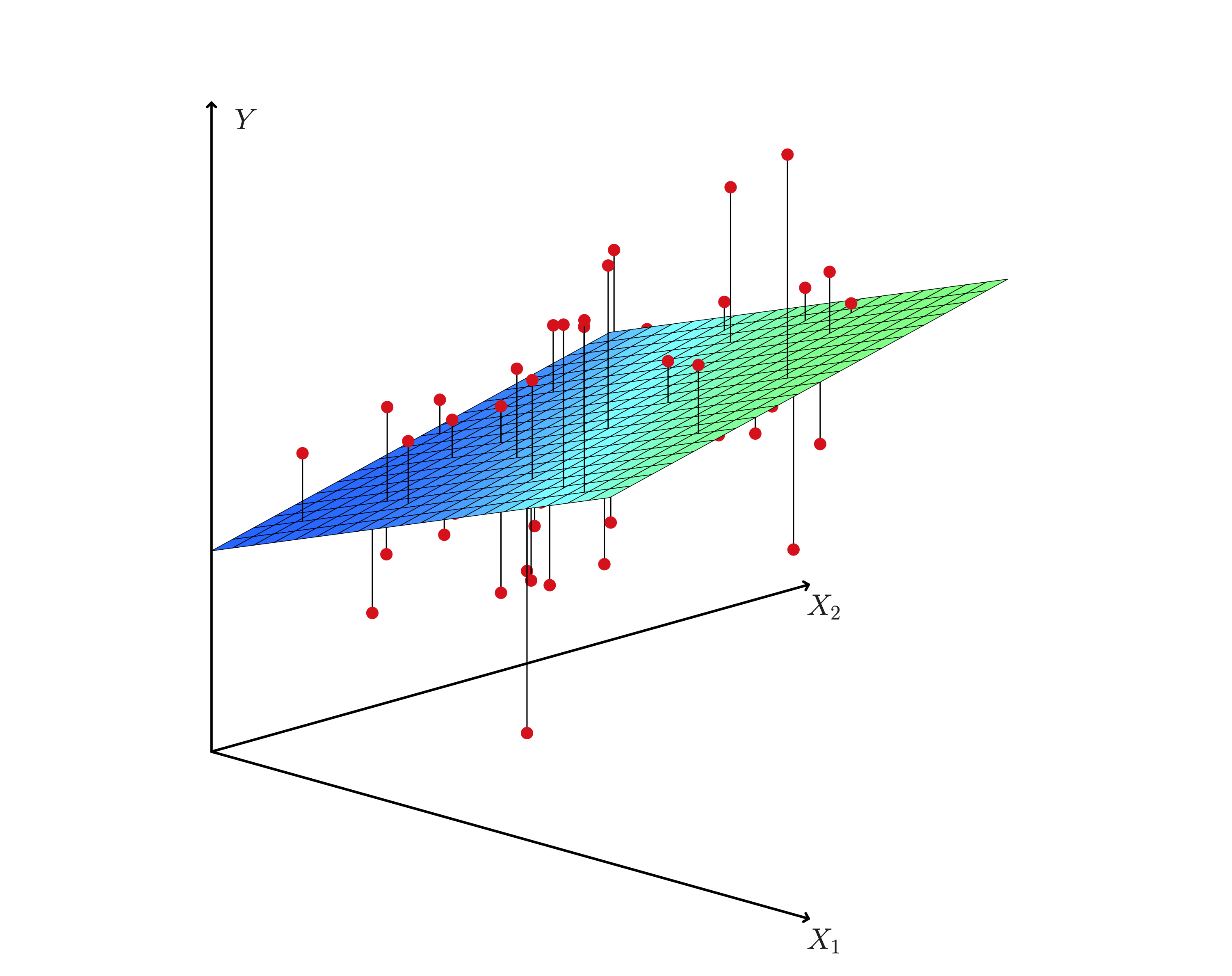
Multiple Regression
- Multiple regression is an extension of simple linear regression to the case of two or more independent variables.
- This allows to look at the relationship between the dependent variable and several independent variables.
- The model is given by:
\[ Y = \beta_0 + \beta_1 X_1 + \beta_2 X_2 + \ldots + \beta_k X_k + \varepsilon \]
Multiple Regression
- The value of multiple regression is that in calculating the effect of on variable, we take into account its variability with respect to other variables.
- We can “control” for the effect of other variables.
- This is especially useful when we really have one variable of interest and other variables are “observables” that are important to control for.
- For instance, if we wanted to understand the effect of SAT on GPA, we would want to control for ACT scores.
Multiple Regression


Least Squares Estimation
- How do we actually find these new coefficients?
- We use the same method as in simple regression: least squares estimation.
- But because we are using multiple variables, this involves doing some matrix algebra.
\[ min \sum_{i=1}^{n} (Y_i - \hat{Y}_i)^2 \]
- In matrix form, the solution is given by:
\[ b = (X'X)^{-1}X'Y \]
\[ \left(X^{\prime} X\right)_{j k}=\sum_{i=1}^n x_{i j} x_{i k} \]
- No need to worry about the details of this formula, but it’s good to know that it exists.
- Note two things:
- \(X'X\) is the variance-covariance matrix of the independent variables.
- \(X'Y\) is the covariance between the dependent variable and the independent variables.
- Similar to the single regression coefficient, but the solution here calculates the variance and covariance between the independent variables with the dependent variable AND the independent variables with each other.
- This allows us to “control” for the effect of other variables.
Least Squares Estimation
Least Squares Estimation
Interpretation of Coefficients
- The interpretation of the coefficients is similar to that of simple regression.
- But now we have to be careful about what the coefficients in relation to the other variables.
Interpretation of Coefficients

- What is the effect of
sat_totalon GPA? - The effect is that a one unit increase in SAT leads to a 0.001 increase in GPA, holding all other variables constant.
- Like a ceteris paribus condition.
Coefficient of Determination
\[ TSS = SSR + ESS \]
\[ \sum_{i=1}^{n} (Y_i - \bar{Y})^2 = \sum_{i=1}^{n} (Y_i - \hat{Y}_i)^2 + \sum_{i=1}^{n} (\hat{Y}_i - \bar{Y})^2 \]
Coefficient of Determination
- Just as before, we can calculate the coefficient of determination, \(R^2\)
\[ R^2 = \frac{SSR}{TSS} = 1 - \frac{ESS}{TSS} \]
Coefficient of Determination
- But what happens to this simple formula when we add more variables?


- The \(R^2\) will always increase when we add more variables, even if they are not significant.
Adjusted R-squared
\[ R^2_{adj} = 1 - \frac{(1 - R^2)(n - 1)}{(n - k - 1)} \]
Assumptions of Multiple Regression
- A0: The relationship between all X’s and Y is linear
- A1: \(E(\varepsilon) = 0\)
- A2: \(E(\varepsilon_i |X_i, \ldots, X_k) = 0\)
- A3: Homoscedasticity, \(Var(\varepsilon_i |X_i, \ldots, X_k) = \sigma^2\)
- A4: No autocorrelation, \(Cov(\varepsilon_i, \varepsilon_j |X_i, \ldots, X_k) = 0\)
- A5: \(\varepsilon_i \sim N(0, \sigma^2)\)
- A6: No multicollinearity, an \(X\) cannot be expressed as a linear combination of other \(X\)’s
Hypothesis Testing: Individual Significance
- Like in simple regression, we can test \(\beta_j = 0\) for each coefficient.
We reject the null hypothesis if:
\[ t_j = \frac{b_j}{SE(b_j)} > t_{n-k-1, \alpha/2} \]
where \(k\) is the number of independent variables and \(n\) is the number of observations.
Other Non-linearities
- Not to be confused with non-linearity in the relationship between the dependent and independent variables.
- We can include non-linearity in the X’s, but not in the effects!
- For instance, we might think that wages rise with age, but they do so more steeply at younger ages and then reach some peak.
- In that case, we can allow for that and test it, by including a quadratic term:
\[ wage = \beta_0 + \beta_1 age + \beta_2 age^2 + \varepsilon \]
- what would be the partial effect of age on wage?
\[ \frac{\partial wage}{\partial age} = \beta_1 + 2 \beta_2 age \]
Non-linearity

Non-linearity: Dummy Variables
- A dummy variable is a variable that takes the value of 1 or 0.
Ex: female = 1 if female, 0 if not
\[ lnwage = \beta_0 + beta_1 \cdot educ + \beta_2 \cdot female + \varepsilon_i \]
How do we interpret this coefficient?
\[ \beta_2 = \frac{\partial E(lnwage| educ,female)}{\partial female} \]
\[ \beta_2 = E(lnwage | educ, female=1) - E(lnwage | educ, female=0) \]
Recall that \(\beta_0\) is where all independent variables are 0. - So \(\beta_0 + \beta_2= E(lnwage | educ, female=1)\)

Categorical Variables as Dummy Variables
- Sometimes we have categorical variables that take on more than two values.
- This might be industry codes, educational attainment, or race.
- In this case, it makes the most sense to create a dummy variable for each category and see the specific effect of each category.
Interpretation
The interpretation of the coefficients is similar to that of a regular dummy variable.
But can we include all categories?
We can’t include all categories because of multicollinearity.
If we include all categories and the categories are mutually exclusive and exhaustive, then we can express one category as a linear combination of the others.
Example:
Industries:
- Agriculture_dummy
- Manufacturing_dummy
- Services_dummy
We KNOW that:
\[ Agriculture_dummy + Manufacturing_dummy + Services_dummy = 1 \]
Interpretation


Interpretation
- This is assumption A6. Stata does not know how to handle multicollinearity, so it will drop one of the categories.
- It breaks down the ability to do the matrix algebra required for finding \(b\).
- But what we happens when we drop a category is that the dropped category becomes the “base” category.
- The coefficients of the other categories are interpreted as the difference between that category and the base category.
- Think about that \(\beta_0\) is when all X’s are 0.
- In this case \(\beta_0\) will be where all X’s are 0 and categorical variable is set at the base category.
Interpretation
- So the interpretation of
hsgradan effect of .24 relative to finishing less than high school.
Interaction Variables
- For our effect on
female, the interpretation is that relative being not female, females earn around 27% less. - That is a level effect. But what if being female also changed the effect of another variable, like education.
- Not only do women make less, on average, but they would also earn less from an extra year of education than men.
- For this we can include an interaction term:
\[ lnwage = \beta_0 + \beta_1 \cdot educ + \beta_2 \cdot female + \beta_3 \cdot female * educ + \varepsilon_i \]
So the partial effect of education on wage is:
\[ \frac{\partial lnwage}{\partial education} = \beta_1 + \beta_3 \cdot female \]
So
\[ \beta_1 \text{ if female =0 } \]
\[ \beta_1 + \beta_3 \text{ if female=1} \]
To test whether the interaction is significant, we can test if \(\beta_3 = 0\).
Hypothesis Test on Several Coefficients
- What is joint significance?
- Essentially, a generalization of the t-test.
- We can test whether a group of coefficients are equal to 0.
Example:
\[ H_0: \beta_2 =0 \text{ and } \beta_3 = 0 \]
\[ H_1: \beta_2 \neq 0 \text{ or } \beta_3 \neq 0 \]
- NOT the same as testing each separately.
- Why?
Hypothesis Test on Several Coefficients
- Involves running two regressions:
- One ASSUMING that the null hypothesis is true (the restricted regression)
- The other is our regression (unrestricted regression)
- Then “comparing” them by explanatory power.
Hypothesis Test on Several Coefficients

Hypothesis Test on Several Coefficients
- Procedure
- Run the unrestricted regression and calculate \(R^2_{unrestricted}\)
- Run the restricted regression and calculate \(R^2_{restricted}\)
- Calculate the F-statistic:
\[ F = \frac{\frac{SSE_u - SSE_r}{m}}{\frac{SSE_r}{n - k - 1}} \]
The test asks if the unrestricted model “does a better job” of explaining the data than the restricted model.
If so, reject the null hypothesis.
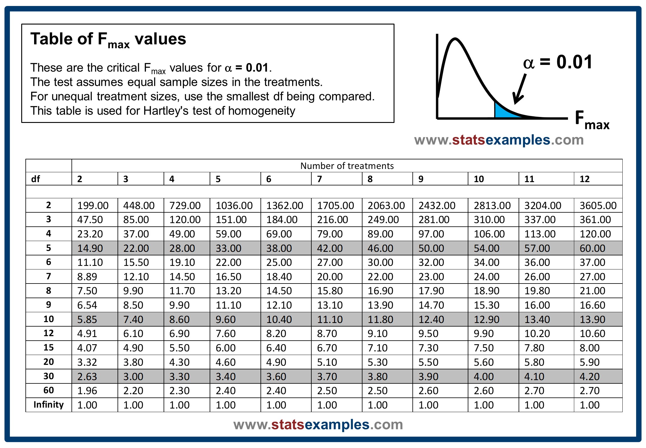
F-Distribution
- The F-distribution is a ratio of two chi-squared distributions.
- The F-distribution is a right-skewed distribution.
Example

Back to the example

Relationship between F-test and \(R^2\)
We can rewrite the F-statistic as:
\[ F = \frac{(R^2_{unrestricted} - R^2_{restricted})/m}{(1 - R^2_{unrestricted})/(n - k - 1)} \]
Can we estimate multiple regression as simple regressions?
- I wasn’t completely truthful before about simple vs. multiple regression.
- We can estimate multiple regression as a series of simple regressions.
- But we have to clever about how we do it.
- Need to take into account the covariances between the independent variables.
- This is called the Frisch-Waugh-Lowell theorem.
Frisch-Waugh-Lowell theorem
Let’s take a look at the following regression:
\[ Y = \beta_0 + \beta_1 X_1 + \beta_2 X_2 + \varepsilon \]
Let’s say that we wanted to estimate the effect of \(X_1\) on \(Y\).
- We can run a regression of \(Y\) on \(X_2\) and get the residuals:
\[ Y = \alpha_0 + \alpha_1 X_2 + \varepsilon_{Y} \]
The residuals in this case are the part of \(Y\) that is not explained by \(X_2\). We have “purged” \(Y\) of the effect of \(X_2\).
- We can also run a regression of \(X_1\) on \(X_2\) and get the residuals: \[ X_1 = \gamma_0 + \gamma_1 X_2 + \varepsilon_{X1} \]
The residuals in this case are the part of \(X_1\) that is not explained by \(X_2\). We have “purged” \(X_1\) of the effect of \(X_2\).
- We can then run a regression of the residuals of \(Y\) on the residuals of \(X_1\):
\[ Y_{res} = \beta_0 + \beta_1 X_{1res} + \varepsilon \]
- This is equivalent to running the original regression.
But!
- The coefficients will be the same, but the standard errors will be different.
- This is because the residuals are not independent of each other.
- The standard errors will be larger because the residuals are correlated.
Nice Trick but… why?
- This is a nice trick, but why would we want to do this?
- With multiple regression, it becomes difficult to visualize the relationship between the dependent and independent variables.
- Simple regression is a 2D plot.
- With FWL, we can visualize the relationship between the dependent variable and one independent variable, while controlling for the other independent variables.