Introduction to Probability

EC031-S26

Aleksandr Michuda

Agenda

• Random Experiments, Counting Rules, and Assigning Probabilities
• Events and Their Probability
• Some Basic Relationships of Probability
• Conditional Probability
• Bayes’ Theorem

Uncertainty

• Statistics and Econometrics is all about quantifying uncertainty
• Any insight always comes with some uncertainty about the result
• This is a natural part of any data analysis
  • In fact if you find something with certainty, there’s probably something wrong!

Probability

• Probability is a numerical measure of the likelihood that an event will occur.
• Probability values are always assigned on a scale from 0 to 1.
• A probability near zero indicates an event is quite unlikely to occur.
• A probability near one indicates an event is almost certain to occur.

Random Experiments and Sample Space

• When understanding probability, you have to understand the sample space over which the probability is calculated
• The sample space for an experiment is the set of all experimental outcomes.
• An experimental outcome is also called a sample point or basic outcome.
• An event is a subset of outcomes

Experiment	Experimental Outcomes	Example Event
Toss a coin	Head, tail	-
Inspect a part	Defective, non-defective	-
Conduct a sale call	Purchase, no purchase	-
Roll a die	1, 2, 3, 4, 5, 6	Roll a number>=5
Play a football game	Win, lose, tie	Win or Tie

An Event in a Sample Space

Draw an event, A, in a sample space!

The Complement

The Complement is all outcomes in S, that are not in A

\[ A' \text{ or } A^{c} \]

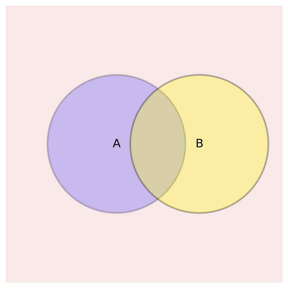
Two Events

Suppose there are two events, A and B.

What is their union?

What is their intersection?

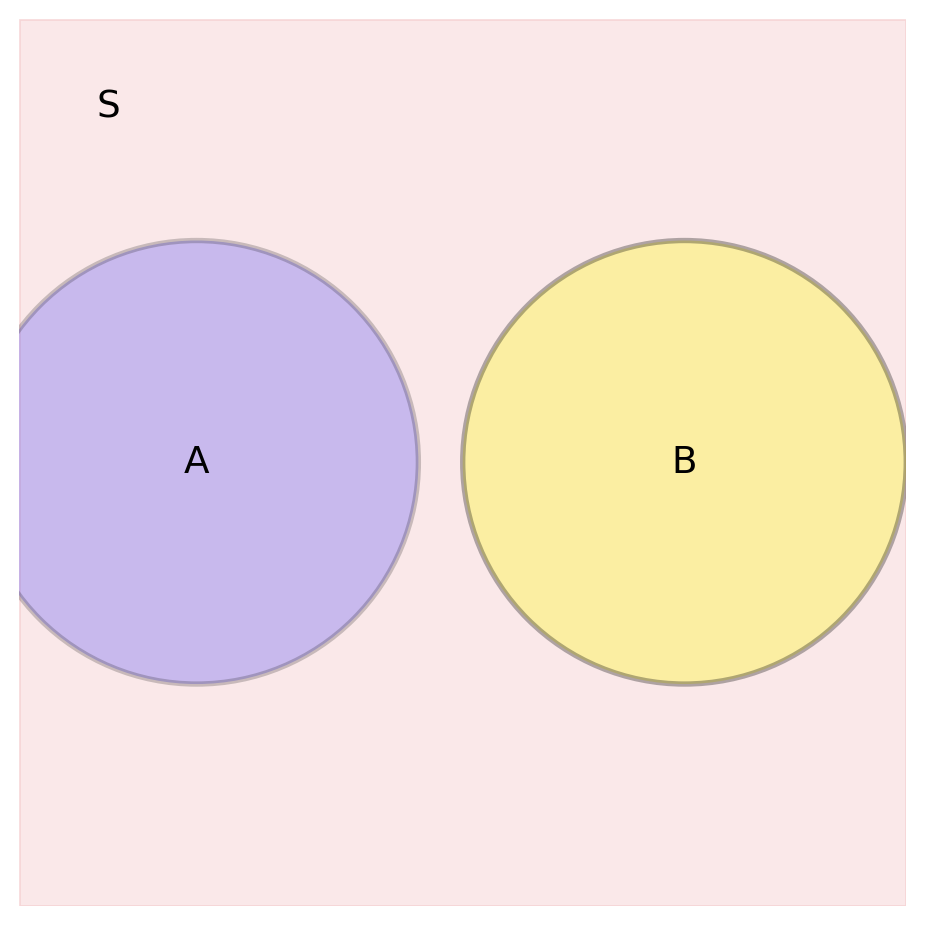
Relationships between Events

• A and B are mutually exclusive if:

• What is a partition of S?

The Axioms

Kolmogorov’s Axioms:

• \(P(A)\geq 0\) : probabilities are non-negative
• \(P(S) = 1\): The probability of all events/the sample space/“something” occurs = 100%

With these two axioms, we can say that a probability is between 0 and 1 (\(0\leq P(A) \leq 1\))

The Addition property:

If events \(A_1 ,...,A_k\) are mutually exclusive, then:

\[ P(A_1 \cup A_2 \cup A_3 \cup ... \cup A_k) = P(A_1) + P(A_2) + ... + P(A_k) = \sum_i^k P(A_i) \]

The Addition Property

• Does not hold if events are NOT mutually exclusive!

Why not?

How does the intersection factor in?

Other Useful Results based on the Postulates

\[ P(A') = 1 - P(A) \tag{1}\]

\[ P(\emptyset) = 0 \tag{2}\]

\[ \text{If } A \subseteq B \rightarrow P(A) \leq P(B) \tag{3}\]

Independence

A and B are independent if:

\[ P(A \cap B) = P(A)P(B) \]

Is this the same as mutually exclusive?

NO, in fact mutually exclusive events are VERY dependent.

If event A occurs, you KNOW event B has not occurred.

Independence vs. Mutual Exclusion

Mutually Exclusive Events

• You can’t be both sitting and standing at the same time
• A traffic light can’t be both red and green simultaneously
• You can’t be both indoors and outdoors at once
• A restaurant can’t be both open and closed at the same moment

Independent Events

• Whether it’s raining in New York doesn’t affect how many likes your latest post receives
• The outcome of a coin flip doesn’t affect the outcome of the next flip
• The number of cars passing by your house doesn’t affect the stock market

Conditioning on an Event

• Often we have situations where our evaluation of the probability of one event (e.g., event A) is changed by the knowledge that some other event (B) has occurred.
• This is called conditioning on an event.
• We have knowledge that an event already occurred
  • Almost like injecting “time” into our probability calculations

Conditional Probability

• Another way to say it is that a conditional probability is a way to “slice” an event by another event
• We know that B has occured, so what is the probability of A occurring in that smaller sample space?

\[ P(A|B) = \frac{P(A \cap B)}{P(B)} \]

Example

Suppose that the probability of majoring in economics is:

\[ P(\text{major}) = 0.21 \]

and the probability of identifying as a democrat is:

\[ P(\text{democrat}) = 0.5 \]

The probability of majoring in econ AND being a democrat is 0.06.

What is \(P(major | democrat)\)?

What is \(P(democrat | major )\)?

Conditioning on Multiple Events

• We can also condition on multiple events

\[ P(A | B, C) = \frac{P(A \cap B \cap C)}{P(B \cap C)} \]

• With corresponding changes to Bayes Theorem and other formulas:

\[ P(A | B, C) = \frac{P(B | A, C)P(A | C)}{P(B | C)} \]

Conditional Independence

Sometime the probability that one event has occurred gives us NO additional information about the likelihood of A occurring.

\[ P(A|B) = P(A) \]

Does Independence Imply Conditional Independence?

• Suppose A and B are independent
  • Are A and B independent, conditional on C?
  • \(P(A \cap B) = P(A)P(B) \rightarrow P(A|C)P(B|C)?\)
• Now suppose that A and B are conditional on C
  • Are A and B independent?
  • \(P(A \cap B|C)=P(A|C)P(B|C) \rightarrow P(A)P(B)?\)

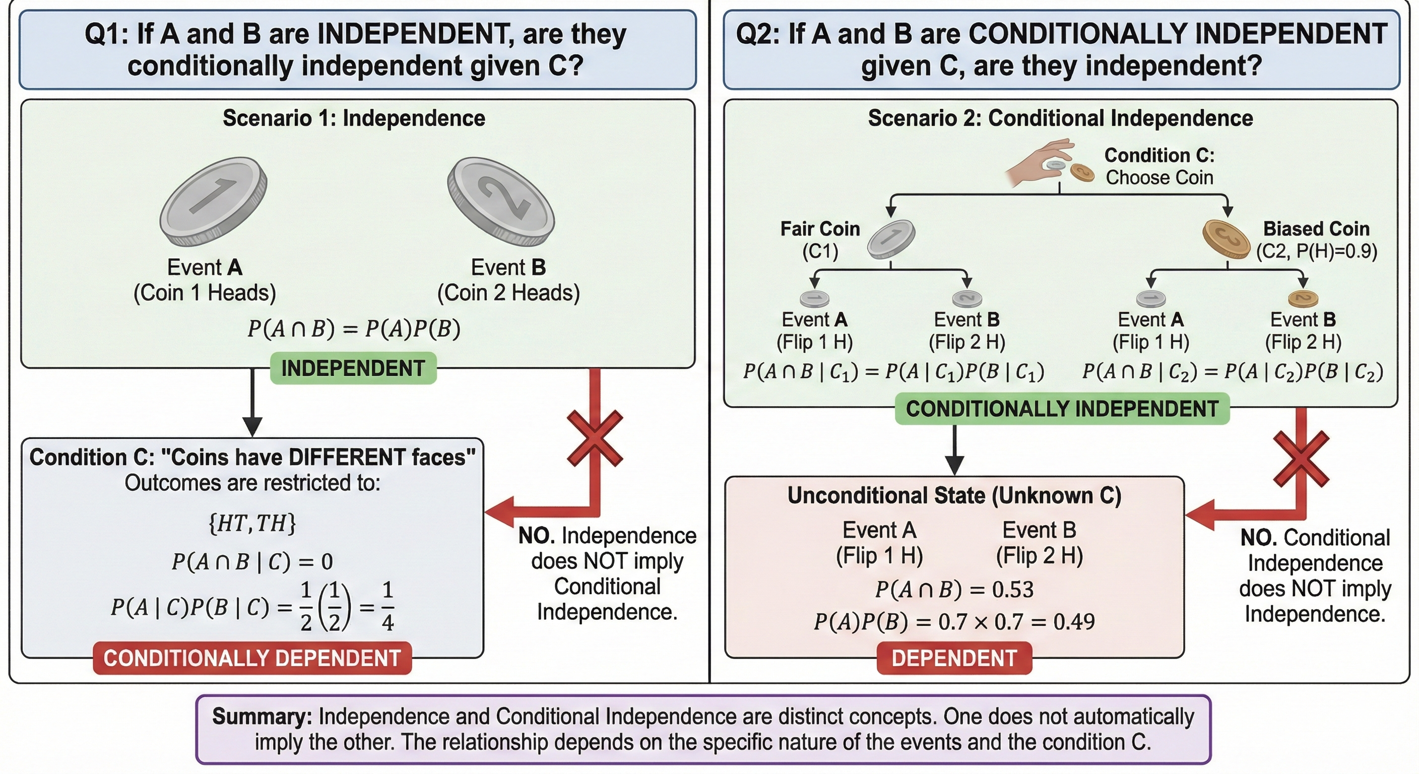
What do we learn?

• In both cases, no!
• In the first case, if A and B are independent, they can still be dependent conditional on C.
• In the second case, if A and B are conditionally independent, they can still be dependent unconditionally.
• This is an important distinction because

Bayes Theorem

• We will soon see the difference between “frequentist” and “Bayesian” statistics.
• Most econometrics is based on “frequentist” statistics
• The basis of Bayesian statistics is based on the idea of prior probabilities, updating of beliefs and forming posterior probabilities based on Bayes Theorem.

Bayes Theorem

• Bayes Theorem is a different way to write conditional probability. It is a way to “flip” the conditioning of probabilities.

\[ P(A|B) = \frac{P(B|A)P(A)}{P(B)} \]

• Where does it come from?

• We can derive it from the definition of conditional probability:

\[ P(A|B) = \frac{P(A \cap B)}{P(B)} \]

• But we can also write:

\[ P(B|A) = \frac{P(B \cap A)}{P(A)} \]

• Rearranging this gives:

\[ P(A \cap B) = P(B|A)P(A) \]

Bayes Theorem

\[ P(A|B) = \frac{P(B|A)P(A)}{P(B)} \]

• So Bayes theorem tell us that we can use what we know about the new information (B) to update our beliefs about A.
• Since we have knowledge about B, we can use that to get a better estimate of A.

Bayesian Thinking

• Bayesian contend that Bayesian thinking and Bayes Theorem is a lot like how people actually think:

flowchart LR
A[I have belief about something] --> B(I am confronted with some information) --> C{I update my beliefs} --> A

And hopefully, I get closer to the “truth”

Bayes Rule/Theorem

• Updating of beliefs is done with the formula:

\[ P(A|B) = \frac{P(B|A)P(A)}{P(B)} \]

Where \(P(B)\) is then calculated using the law of total probability:

\[ P(B) = P(A)P(B|A) + (1-P(A))P(B|\neg A) \]

or with more A events: \(P(B) = \sum_i^k P(A_i)P(B|A_i)\) is the Law of Total Probability

The Law of Total Probability

The Law of Total Probability is the idea that to get the probability of an event, you can sum up lots of conditional probabilities weighted by what you’re conditioning on.

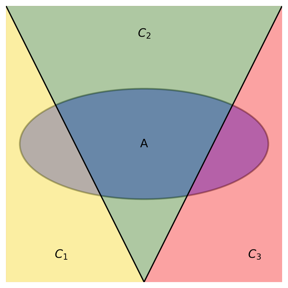
\[ P(A) = P(A \cap C_1) + P(A \cap C_2) + P(A \cap C_3) \]

or

\[ P(A) = P(C_1)P(A|C_1) + P(C_2)P(A|C_2) + P(C_3)P(A|C_3) \]

Example

Let’s say that we have some preliminary information about whether the senator of a state will win an election:

\[ P(win) = .7 \]

\[ P(lose) = 1 - P(win) = .3 \]

New Information

Some news comes in that suggests the Senator is a cat person. This takes over the news cycle for 48 hours as cat food manufacturers begin investing heavily in the campaign, while the Dog lobby begins frantically carrying out opposition research. How should we update our beliefs on the outcome of the election?

All we know is that based on previous data, after winning an election, candidates tended to be cat people with probability .2 and candidates tended to be cat people after losing an election with probability .9.

\[ P(\text{cat person} | win) = .2 \]

\[ P(\text{cat person} | lose) = .9 \]

Solving this

Our goal is then to find the new probability, \(P(win | cat person)\).

\[ P(win | \text{cat person}) = \frac{P(\text{cat person} | win)P(win)}{P(\text{cat person})} \]

We know the probability of winning and the conditional probability in the numerator, how do we get the probability of a cat person?

P(cat person)

To get \(P(\text{cat person})\), we just use the law of total probability:

\[ \begin{split} P(\text{cat person}) &= P(win)P(\text{cat person} | win) + P(lose) P(\text{cat person} | lose) \\ &= .7(.2) + .3(.9) = .14 + .27 \\ &=.41 \end{split} \]

Final Calculation

Finally, we just plug that in:

\[ P(win | \text{cat person}) = \frac{.7(.2)}{.41} = .34 \]

So based on this information, we have gone from from the probability of winning of .7 \(\rightarrow\) .34.

Don’t be a cat person if you have political ambitions!

Bayesian Networks

• Graphical models that represent the probabilistic relationships among a set of variables.
• Can model more complex systems where variables are interdependent and uncertainty is present.
• Each node in the network represents a random variable, and the directed edges between nodes represent conditional dependencies.
• Bayesian networks are widely used in various fields, including machine learning, artificial intelligence, and decision analysis, to perform tasks such as inference, prediction, and decision-making under uncertainty.
• We will not go in-depth on this, but the basics of Bayesian networks are useful for understanding causal inference later in the course.

Example

• A Bayesian network encodes information about the joint probability distribution of a set of random variables.
• The information from the nodes (variables) and edges (dependencies) can be used to break down complex joint probability distributions into simpler conditional probabilities.

graph LR
    T[Tax Cuts]
    Y[GDP Growth]
    S[Sentiment]
    I[Investment]

    T --> I 
    S --> I
    I --> Y

• We can see here that tax cuts affect investment in the economy, but it also might change sentiment about investment. Investment then feeds into GDP growth.

Bayesian Networks

• The joint probability distribution for this network is:

\[ P(T, Y, S, I) \]

• This is the same as saying \(P(T \cap Y \cap S \cap I)\), which is the probability of all of these events happening together.
• How do we break this up using the definition of conditional probability?

\[ P(T, S, I, G) = P(T) \cdot P(S|T) \cdot P(I|T, S) \cdot P(G|T, S, I) \]

• But we can break this down into conditional probabilities using the structure of the network:

\[ P(T, Y, S, I) = P(T)P(S)P(I|T,S)P(Y|I) \]

• Let’s break this down
• If all these probabilities were independent of each other, we could write it as:

\[ P(T, Y, S, I) = P(T)P(S)P(I)P(Y) \]

• But the network here tells us that there are dependencies between the variables.
• We know that the marginal probability of tax cuts, \(P(T)\) is independent of everything else.
• So:

\[ P(T|Y,S,I) = P(T) \]

• Sentiment is also independent of everything else:

\[ P(S|T,Y,I) = P(S) \]

• Investment depends on tax cuts and sentiment, but is independent of GDP growth:

\[ P(I|T,Y,S) = P(I|T,S) \]

• Finally, GDP growth depends only on investment:

\[ P(Y|T,S,I) = P(Y|I) \]

Example: Rain and Wet Grass

One day you wake up, and you look out the window at your lawn. You see that the grass is wet. You wonder whether it rained last night. You know that you live dry place, and the probability of rain is about 20%. When it rains, the probability that the grass gets wet is 90%. However, sometimes the morning dew makes the grass wet, even if it didn’t rain. The probability of dew making the grass wet is 20%. So now you ask, given that the grass is wet, what is the probability that it rained last night?

• This leads to a pretty simple Bayesian network:

graph LR
    R[Rain]
    G[Wet Grass]

    R --> G

• This can be solved in the same way that we solved the previous example with the senator and cat people.

• Let R = 1 if it rained, 0 otherwise

• Let G = 1 if the grass is wet, 0 otherwise

• We know that: \[ P(R=1) = 0.2 \]

\[ P(G=1|R=1) = 0.9 \]

\[ P(G=1|R=0) = 0.2 \]

• We want to find \(P(R=1|G=1)\)

Using Bayes Theorem:

\[ P(R=1|G=1) = \frac{P(G=1|R=1)P(R=1)}{P(G=1)} \]

• We need to find \(P(G=1)\) using the law of total probability:

\[ \begin{split} P(G=1) &= P(R=1)P(G=1|R=1) + P(R=0)P(G=1|R=0) \\ &= 0.2(0.9) + 0.8(0.2) = 0.18 + 0.16 = 0.34 \end{split} \]

• Now we can plug everything in:

\[ P(R=1|G=1) = \frac{0.9(0.2)}{0.34} = \frac{0.18}{0.34} \approx 0.5294 \]

More Complicated Example

• What if we also have a sprinkler?
• Let’s say that the sprinkler is on a timer, so it doesn’t “know” if it has rained or not.
• Let’s say that morning dew is not a factor anymore.
• What does this imply about what the resulting would look like?
• What would it look like if the sprinkler had a sensor to know if it had rained?

graph LR
    R[Rain]
    S[Sprinkler]
    W[Wet Grass]
    R --> W
    S --> W

More Complicated Example

• So let’s say you wake up and see that the grass was wet. It isn’t clear whether it was rain or the sprinkler that made the grass wet.
• The probability of rain is still 20%.
• The probability that the sprinkler is on is 10%.
• We can also say that if it rains OR the sprinkler is on, the probability that the grass is wet is 100%.
  • What does this mean in terms of probabilities?
  • If even one of those events happens, the grass is wet with probability 1.
  • So \(P(W=1|R=1,S=0) = 1\), \(P(W=1|R=0,S=1) = 1\), and \(P(W=1|R=1,S=1) = 1\)
  • But if neither happens, the grass is dry with probability 1.
  • So \(P(W=1|R=0,S=0) = 0\)
  • So what’s the probability of it being wet (\(P(W=1)\))?

The probability of the grass being wet

• We can use the law of total probability again:

\[ \begin{split} P(W=1) &= P(R=1,S=1)P(W=1|R=1,S=1) + P(R=1,S=0)P(W=1|R=1,S=0) \\ &+ P(R=0,S=1)P(W=1|R=0,S=1) + P(R=0,S=0)P(W=1|R=0,S=0) \\ &= (0.2)(0.1)(1) + (0.2)(0.9)(1) + (0.8)(0.1)(1) + (0.8)(0.9)(0) \\ &= 0.02 + 0.18 + 0.08 + 0 = 0.28 \end{split} \]

Or what’s an easier way to do this?

• It’s easier to find the probability of it being dry, and subtract from 1:

\[ P(W=0) = P(R=0,S=0)P(W=0|R=0,S=0) = (0.8)(0.9)(1) = 0.72 \]

• So then:

\[ P(W=1) = 1 - P(W=0) = 1 - 0.72 = 0.28 \]

More Complicated Example

• So what’s the probability that it rained, given that the grass is wet?

\[ P(R=1|W=1, S) \]

• But we can simplify this to:

\[ P(R=1|W=1) \]

To do this we need to use Bayes Theorem again:

\[ P(R=1|W=1) = \frac{P(W=1|R=1)P(R=1)}{P(W=1)} \]

• What is the first term equal to?

• We know each of the terms:

\[ P(W=1|R=1) = \frac{1*.2}{.28} \approx .7143 \]

• The probability of rain jumps from 20% to over 71% just because we see the grass is wet.

Explaining Away

• Now suppose we also know that the sprinkler was on.

• How does this change our belief about whether it rained?

• What is \(P(R=1|W=1,S=1)\)?

• Using Bayes Theorem again:

\[ P(R=1|W=1,S=1) = \frac{P(W=1|R=1,S=1)P(R=1)}{P(W=1|S=1)} \]

• Using what we know about the independence of R and S, we can find the denominator:

\[ P(R=1 |W=1, S=1) = P(R=1|W=1) = \frac{1*.2}{1} \]

• By knowing that the sprinkler was on, the probability of rain drops back to 20% because we found evidence of another cause of the wet grass.
• This is called “explaining away” in Bayesian networks.