Text(0.5, 1.0, '$\\hat{\\theta} = \\bar{X}$ (mean: 0.022)')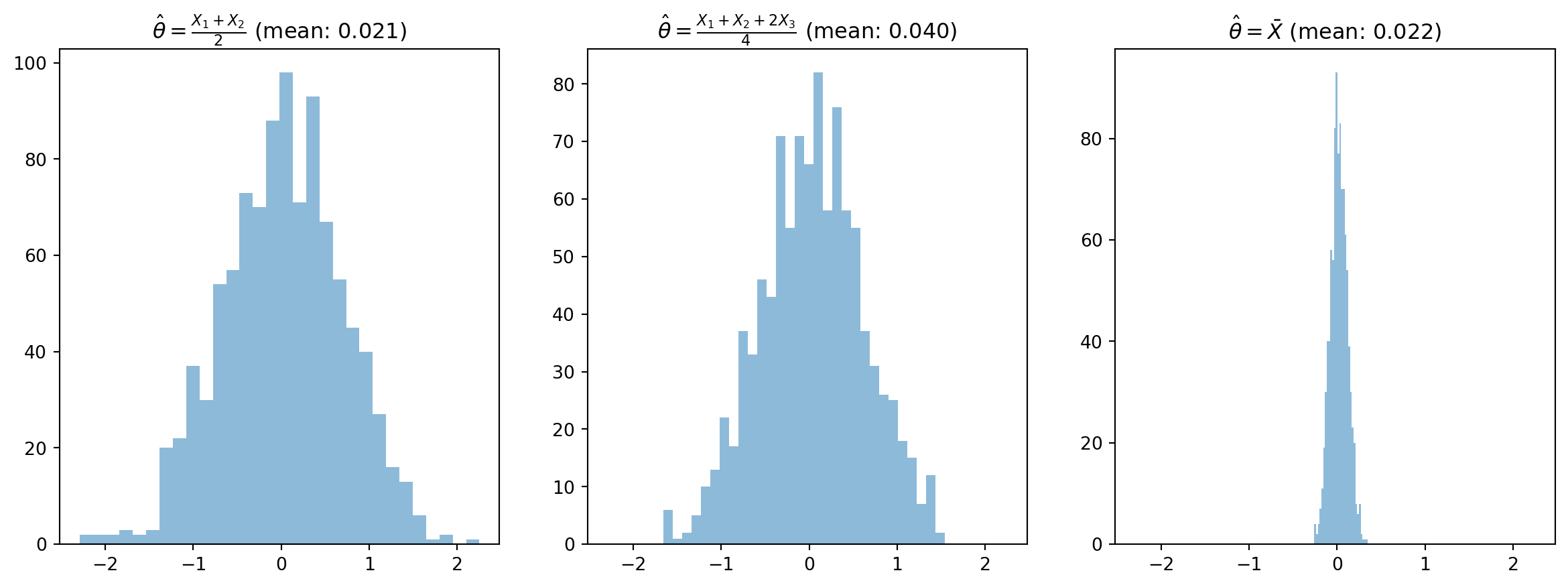
EC031-S26
Finite Sample Properties
\[ E(\hat{\theta}) = \theta \]
Asymptotic Properties
There are many estimators for a single population parameter.
Text(0.5, 1.0, '$\\hat{\\theta} = \\bar{X}$ (mean: 0.022)')
\[ E(\hat{\theta}) = \theta \]
\[ E(\bar{X}) = E(\frac{1}{n} \sum_{i=1}^{n} X_i) = \frac{1}{n} \sum_{i=1}^{n} E(X_i) = \frac{1}{n} \sum_{i=1}^{n} \mu = \mu \]
\[ E(\hat{\theta}) = E(\frac{X_1 + X_2}{2}) \]
Note
\[ E(\hat{\theta}) = E(\frac{X_1 + X_2}{2}) = \frac{1}{2}E(X_1) + \frac{1}{2}E(X_2) = \mu \]
\[ E(\hat{\theta}) = E(\frac{X_1 + X_2 + 2X_3}{4}) \]
Note
\[ E(\hat{\theta}) = E(\frac{X_1 + X_2 + 2X_3}{4}) = \frac{1}{4}E(X_1) + \frac{1}{4}E(X_2) + \frac{1}{2}E(X_3) = \mu \]
\[ E(\hat{\theta}) = E(\frac{X_1 + X_2 + 3X_3}{4}) \]
Note
\[ E(\hat{\theta}) = E(\frac{X_1 + X_2 + 3X_3}{4}) = \frac{1}{4}E(X_1) + \frac{1}{4}E(X_2) + \frac{3}{4}E(X_3) = \frac{5}{4} \mu \]
Biased!
What’s the variance of all of our estimators?
\[ Var(\bar{X}) = Var(\frac{1}{n} \sum_{i=1}^{n} X_i) = \frac{1}{n^2} \sum_{i=1}^{n} Var(X_i) = \frac{1}{n^2} \sum_{i=1}^{n} \sigma^2 = \frac{\sigma^2}{n} \]
What assumption are we making between the \(X_i\)?
\[ Var(\hat{\theta}) = Var(\frac{X_1 + X_2}{2}) \]
Note
\[ Var(\hat{\theta}) = Var(\frac{X_1 + X_2}{2}) = \frac{1}{4}Var(X_1) + \frac{1}{4}Var(X_2) = \frac{\sigma^2}{2} \]
\[ Var(\hat{\theta}) = Var(\frac{X_1 + X_2 + 2X_3}{4}) \]
Note
\[ Var(\hat{\theta}) = Var(\frac{X_1 + X_2 + 2X_3}{4}) = \frac{1}{16}Var(X_1) + \frac{1}{16}Var(X_2) + \frac{4}{16}Var(X_3) = \frac{9\sigma^2}{16} \]
\[ Var(\hat{\theta}) = Var(\frac{X_1 + X_2 + 3X_3}{4}) \]
Note
\[ Var(\hat{\theta}) = Var(\frac{X_1 + X_2 + 3X_3}{4}) = \frac{1}{16}Var(X_1) + \frac{1}{16}Var(X_2) + \frac{9}{16}Var(X_3) = \frac{11\sigma^2}{16} \]
Below is a table of all of the variances we calculated:
| Estimator | Variance |
|---|---|
| \(\bar{X}\) | \(\frac{\sigma^2}{n}\) |
| \(\frac{X_1 + X_2}{2}\) | \(\frac{\sigma^2}{2}\) |
| \(\frac{X_1 + X_2 + 2X_3}{4}\) | \(\frac{9\sigma^2}{16}\) |
| \(\frac{X_1 + X_2 + 3X_3}{4}\) | \(\frac{11\sigma^2}{16}\) |
For the same \(n\), the mean is always the lowest variance estimator!
\[ MSE(\hat{\theta}) = E((\hat{\theta} - \theta)^2) \]
If you do some math, you can find that the MSE can be decomposed into two parts:
\[ MSE(\hat{\theta}) = Var(\hat{\theta}) + Bias(\hat{\theta})^2 \]
Note
\[ MSE(\hat{\theta}) = E((\hat{\theta} - \theta)^2) \]
\[ = E((\hat{\theta} - E(\hat{\theta}) + E(\hat{\theta}) - \theta)^2) \]
\[ = E((\hat{\theta} - E(\hat{\theta}))^2) + E(E(\hat{\theta}) - \theta)^2 + 2E((\hat{\theta} - E(\hat{\theta}))(E(\hat{\theta}) - \theta)) \]
\[ = Var(\hat{\theta}) + Bias(\hat{\theta})^2 \]
\[ \text{Estimate} \pm \text{Margin of Error} \]
The question we want to answer is, what do the lower and upper bounds of the confidence interval have to be in order for me to be \(1-\alpha\) confident that the true population mean is within this interval?
\[ P(LB \leq \mu \leq UB) = 1 - \alpha \]
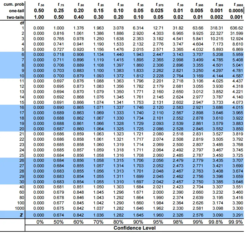
Since we know that \(z\) is a standard normal distribution, we can use the quantiles of the standard normal distribution to find the bounds.
So we want to find a symmetric interval around the sample mean such that:
\[ P(-z^* \leq z \leq z^*) = 1 - \alpha \]
We can get a symmetric bound by just taking \(\alpha/2\) on each side.
Once I find \(z^*\), I can define the probability fully:
\[ P(-z^*_{\alpha/2} \leq \frac{\bar{x}-\mu}{\frac{\sigma}{\sqrt{n}}} \leq z^*_{\alpha/2}) = 1 - \alpha \]
Important
In this case, we are going to assume that we know \(\sigma\)!
Now, with some manipulation, we can find the confidence interval:
\[ P(-z^*_{\alpha/2} \leq \frac{\bar{x}-\mu}{\frac{\sigma}{\sqrt{n}}} \leq z^*_{\alpha/2}) = 1 - \alpha \]
\[ P(-z^*_{\alpha/2} \frac{\sigma}{\sqrt{n}} \leq \bar{x}-\mu \leq z^*_{\alpha/2} \frac{\sigma}{\sqrt{n}}) = 1 - \alpha \]
\[ P(\bar{x} - z^*_{\alpha/2} \frac{\sigma}{\sqrt{n}} \leq \mu \leq \bar{x} + z^*_{\alpha/2} \frac{\sigma}{\sqrt{n}}) = 1 - \alpha \]
\[ CI = \bar{x} \pm z^*_{\alpha/2} \frac{\sigma}{\sqrt{n}} \]
jStat = require("https://cdn.jsdelivr.net/npm/jstat@latest/dist/jstat.min.js");

//Create array for x-axis values
viewof alpha = Inputs.range([0.01, 0.99], {
    step: 0.01,
    value: 0.95,
    label: "Confidence Level (1-α)"
})

function normalPDF(x) {
    return (1 / (Math.sqrt(2 * Math.PI))) * Math.exp(-0.5 * ((x) / 1) ** 2);
}


zScore = -1 * jStat.normal.inv((1-alpha)/2, 0, 1)

Plot.plot({
    width: 800,
    height: 400,
    x: {
        domain: [-4, 4]
    },
    y: {
        domain: [0, 0.45]
    },
    marks: [
        Plot.line(d3.range(-4, 4, 0.01).map(x => ({x, y: normalPDF(x)})), {x: "x", y: "y"}),
        Plot.areaY(d3.range(-4, -zScore, 0.01).map(x => ({x, y: (1 / (1 * Math.sqrt(2 * Math.PI))) * Math.exp(-0.5 * ((x - 0) / 1) ** 2)})), {x: "x", y: "y", fillOpacity: 0.3}),
        Plot.areaY(d3.range(zScore, 4, 0.01).map(x => ({x, y: (1 / (1 * Math.sqrt(2 * Math.PI))) * Math.exp(-0.5 * ((x - 0) / 1) ** 2)})), {x: "x", y: "y", fillOpacity: 0.3}),
        Plot.ruleX([-zScore, zScore])
    ]
})Suppose \(x\) is a random variable reflecting the hours of sleep a student gets per week. \(x\) has an unknown \(\mu\) and a know \(\sigma\) of 16.
Suppose you take a random sample of 64 students and they averaged 45 hours of sleep per week.
Construct a 90% confidence interval for \(\mu\)
Answer
\[ CI = \bar{x} \pm z^*_{\alpha/2} \frac{\sigma}{\sqrt{n}} \]
\[ CI = 45 \pm 1.645 \frac{16}{\sqrt{64}} \]
\[ CI = 45 \pm 3.29 \]
Note that as \(n\) increases, the confidence interval decreases!
\[ P(z \leq z^*) = 1 - \alpha \]
So our critical value is just all that are one side.
Our confidence interval is then:
\[ [\bar{x} - z^*_{\alpha} \frac{\sigma}{\sqrt{n}}, \infty] \]
or
\[ [-\infty, \bar{x} + z^*_{\alpha} \frac{\sigma}{\sqrt{n}}] \]
Suppose \(x\) is a random variable reflecting the hours of sleep a student gets per week. \(x\) has an unknown \(\mu\) and a know \(\sigma\) of 16. Suppose you take a random sample of 64 students and they averaged 45 hours of sleep per week. Construct a 90% right-sided confidence interval for \(\mu\).
Answer
\[ CI = 45 + 1.28 \frac{16}{\sqrt{64}} \]
\[ CI = [45 - 2.56, \infty] \]
\[ s^2 = \frac{1}{n-1} \sum_{i=1}^{n} (X_i - \bar{X})^2 \]
Why this?
Because we know that \(s^2\) is an unbiased estimator of \(\sigma^2\)!
Note
Show that \(E(s^2) = \sigma^2\)
\[ E(s^2) = E(\frac{1}{n-1} \sum_{i=1}^{n} (X_i - \bar{X})^2) \]
\[ = \frac{1}{n-1} \sum_{i=1}^{n} E((X_i - \bar{X})^2) \]
\[ = \frac{1}{n-1} \sum_{i=1}^{n} E((X_i - \mu + \mu - \bar{X})^2) \]
\[ = \frac{1}{n-1} \sum_{i=1}^{n} E((X_i - \mu)^2 + 2(X_i - \mu)(\mu - \bar{X}) + (\mu - \bar{X})^2) \]
\[ = \frac{1}{n-1} \sum_{i=1}^{n} E((X_i - \mu)^2) + 2E(X_i - \mu)E(\mu - \bar{X}) + E(\mu - \bar{X})^2 \]
Finish this…
Tip
The statistic using \(s\) is actually a ratio of a Normally distributed random variable and a \(\chi^2\) distributed random variable. This ratio is called the \(t\) distribution.
So rather than using a normal distribution to calculate critical values, we need to use a t-distribution with \(n-1\) degrees of freedom.
\[ E(\bar{p})=E(\frac{\sum_i x_i}{n}) = \frac{1}{n}\sum_i E(x_i) = \frac{1}{n} np = p \]
Political Science Inc. (PSI) specializes in voter polls and surveys designed to keep political office seekers informed of their position in a race.
Using telephone surveys, PSI interviewers ask registered voters who they would vote for if the election were held that day.
In a current election campaign, PSI has just found that 220 registered voters, out of 500 contacted, favor a particular candidate. PSI wants to develop a 95% confidence interval estimate for the proportion of the population of registered voters that favor the candidate.
The confidence interval is:
\[ CI = \bar{p} \pm z^*_{\alpha/2} \sqrt{\frac{\bar{p}(1-\bar{p})}{n}} \]
\[ CI = 0.44 \pm 1.96 \sqrt{\frac{0.44(1-0.44)}{500}} \]
\[ CI = 0.44 \pm 0.044 \]
\[ m = z^*_{\alpha/2} \frac{\sigma}{\sqrt{n}} \]
Meaning that we can solve for \(n\):
\[ n = (\frac{z^*_{\alpha/2} \sigma}{m})^2 \]
This is what’s called a power analysis, which is very popular when designing experiments.
Again we have the \(\sigma\) problem, however, it is in this case, that the only way to get around it is to use some value that makes sense based on the context.
You might: