Inference about Means with Two Populations

Aleksandr Michuda

Agenda

Inferences about the Difference between Populations with known $\sigma$s.
Inferences about the Difference between Populations with unknown $\sigma$s.
Inference about the Difference between two population means
Inference about the Difference between two population proportions

Difference in Means

The difference in means is a useful way to compare two populations affected by some “treatment”
In a randomized experiment, one group receives the treatment and the other is a control group
Comparing the means between this groups gives the average treatment effect which is a measure of impact

graph TD
    A[Population 1] --> B[Sample 1]
    A --> C[Sample 2]
    B --> D[Mean 1]
    C --> E[Mean 2]
    D --> F[Difference]
    E --> F

Difference in Means

The population with the treatment and the control are then said to have different population means
Suppose you collect data on a treatment and control group and want to check if the treatment was successful.
The control population has a population mean of $\mu_c$ and the treatment population has a population mean of $\mu_t$
How would check if the treatment was successful?
$\mu_t - \mu_c$

Difference in Means

You collect some data to estimate the population means
You collect $n_c$ observations from the control group and $n_t$ observations from the treatment group
You calculate the sample means $\bar{x}_c$ and $\bar{x}_t$
Let’s say for simplicity, you know the population standard deviations $\sigma_c$ and $\sigma_t$
You could check their difference:

\[ \bar{X}_t - \bar{X}_c \]

Difference in Means

Is this estimator of the difference unbiased?

\[ E(\bar{X}_t - \bar{X}_c) = E(\bar{X}_t) - E(\bar{X}_c) = \mu_t - \mu_c \]

Is that enough?

Central Limit Theorem

We’ve seen that the sample mean is normally distributed, what about the difference of means?
Well it turns out that the sum of normal distributions is also normal.
- Proof is omitted…

The Variance of the Difference in Means

Now that we know that $\bar{X}_t - \bar{X}_c$ is normally distributed, we also know that with a z-score transformation, we will have a standard normal and we can use it to generate confidence intervals and hypothesis tests
We already know the expected value of the difference in means, what about the variance?

\[ Var(\bar{X}_t - \bar{X}_c) = Var(\bar{X}_t) + (-1)^2Var(\bar{X}_c) = \frac{\sigma_t^2}{n_t} + \frac{\sigma_c^2}{n_c} \]

Difference in Means

Now we know that:

\[ \bar{X}_t - \bar{X}_c \sim N(\mu_t - \mu_c, \sqrt{\frac{\sigma_t^2}{n_t} + \frac{\sigma_c^2}{n_c}}) \]

or that:

\[ \frac{\bar{X}_t - \bar{X}_c - (\mu_t - \mu_c)}{\sqrt{\frac{\sigma_t^2}{n_t} + \frac{\sigma_c^2}{n_c}}} \sim N(0, 1) \]

Confidence Intervals

We can use the standard normal distribution to generate confidence intervals for the difference in means
The confidence interval is given by:

\[ (\bar{X}_t - \bar{X}_c) \pm z_{\alpha/2}\sqrt{\frac{\sigma_t^2}{n_t} + \frac{\sigma_c^2}{n_c}} \]

Where $z_{\alpha/2}$ is the critical value for the standard normal distribution
Same as we’ve already discussed
With $\alpha$ our desired level of significance.

Two-tailed Tests

We can also use the standard normal distribution to generate hypothesis tests for the difference in means

The null hypothesis for a two-tailed test is:

\[ H_0: \mu_t - \mu_c = D_0 \]

for some difference $D_0$ (but usually 0)

The alternative hypothesis is:

\[ H_1: \mu_t - \mu_c \neq D_0 \]

One-tailed tests

Sometimes you want to make sure that the difference was positive or negative
If the treatment is supposed to improve outcomes, you might want to see if the treatment group has a higher mean

The null hypothesis for a right-tailed test is:

\[ H_0: \mu_t - \mu_c <= D_0 \]

The alternative hypothesis is:

\[ H_1: \mu_t - \mu_c > D_0 \]

For a left-tailed test:

\[ H_0: \mu_t - \mu_c >= D_0 \]

\[ H_1: \mu_t - \mu_c < D_0 \]

$\sigma$ Unknown

Once again, though, we do not know the population standard deviations
So we must use the sample standard deviations instead
This changes the distribution of the difference in means
The distribution is now a t-distribution
But degrees of freedom are more involved

The t-distribution

The degrees of freedom for a difference in means is:

\[ df = \frac{(\frac{s_t^2}{n_t} + \frac{s_c^2}{n_c})^2}{\frac{(\frac{s_t^2}{n_t})^2}{n_t - 1} + \frac{(\frac{s_c^2}{n_c})^2}{n_c - 1}} \]

Why? Previously we just had $n-1$.

The issue comes in adding up the variance of the two distributions

Previously the issue with the unknown $\sigma$ problem was that the test statistic (or z-score transformation) was the ratio of a normal and a chi-squared distribution.

Now the test statistic is the ratio of a normal and a linear combination of chi-squared distributions ($k_i s_i^2 + ... + k_n s_n^2$).

In this case, we need to use an approximation called the Welch-Satterthwaite approximation

This gives an approximate chi-squared distribution for this kind of sum of standard deviations.

Degrees of Freedom

Note that if the sample sizes are equal, then the degrees of freedom are just $n_t + n_c - 2$ or $2n-2$.

Example:

Suppose you are interested in the effect of a new drug on blood pressure
You collect data on two groups of patients
- The control group receives a placebo
- The treatment group receives the drug
You collect data on the blood pressure of the patients in both groups
You want to see if the drug has an effect on blood pressure

Example:

You collect data on 22 patients in the control group and 20 patients in the treatment group
The sample means are $\bar{x}_c = 120$ and $\bar{x}_t = 110$
The sample standard deviations are $s_c = 10$ and $s_t = 15$
You want to test if the drug has an effect on blood pressure at the 5% significance level of a two-tailed test.

Example:

The null hypothesis is that the drug has no effect on blood pressure
The alternative hypothesis is that the drug has an effect on blood pressure

\[ H_0: \mu_t - \mu_c = 0 \]

\[ H_1: \mu_t - \mu_c \neq 0 \]

Example:

The difference in means is:

\[ \bar{x}_t - \bar{x}_c = 110 - 120 = -10 \]

The standard error is:

\[ \sqrt{\frac{s_t^2}{n_t} + \frac{s_c^2}{n_c}} = \sqrt{\frac{15^2}{20} + \frac{10^2}{20}} = 4.03 \]

The degrees of freedom are:

\[ \frac{(\frac{s_t^2}{n_t} + \frac{s_c^2}{n_c})^2}{\frac{(\frac{s_t^2}{n_t})^2}{n_t - 1} + \frac{(\frac{s_c^2}{n_c})^2}{n_c - 1}} \]

\[ \frac{(\frac{15^2}{22} + \frac{10^2}{20})^2}{\frac{(\frac{15^2}{22})^2}{22 - 1} + \frac{(\frac{10^2}{20})^2}{20 - 1}} = 32.635 \]

So we use the lower number for df, 32.

The critical value for a two-tailed test with 47 degrees of freedom is T-TABLE

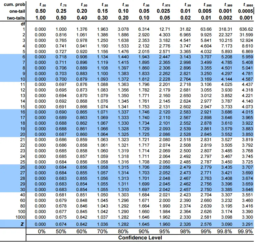
$\approx 2.042$

Example:

The t-score is:

\[ \frac{\bar{x}_t - \bar{x}_c}{\sqrt{\frac{s_t^2}{n_t} + \frac{s_c^2}{n_c}}} = \frac{-10}{3.97} = -2.52 \]

is less than -2.01, so we reject the null hypothesis.

Example:

The p-value is:

\[ 2*P(T_{47} < -2.52) = 0.015 \]

Example:

The p-value is less than 0.05, so we reject the null hypothesis
The drug has an effect on blood pressure

Example:

The confidence interval is:

\[ -10 \pm 2.01*3.97 = -10 \pm 8.0 \]

The confidence interval is (-18, -2)

Confidence Intervals not Crossing

If the confidence intervals for the means do not cross, then the difference in means is statistically significant
But it doesn’t mean that if they do cross, the difference is not significant.
Redo this previous example

Example:

The confidence interval for the control group is (with df=21):

\[ 120 \pm 2.080*\frac{10}{\sqrt{22}} = 120 \pm 4.03 \]

The confidence interval for the treatment group is:

\[ 110 \pm 2.093*\frac{15}{\sqrt{20}} = 110 \pm 6.6 \]

Example:

The confidence interval for the control group is (115.97, 124.03)
The confidence interval for the treatment group is (103.4, 116.6)

The confidence intervals cross, but the difference in means is still significant.

Summary

The key here is that it ultimately depends on the variability of each distribution.

Example: Deworming

Worm infections (hookworm, roundworm, whipworm, schistosomiasis) affect over 1 billion people, mostly in developing countries.
Infections cause fatigue, malnutrition, and school absenteeism.

Economic & Policy Implications

Why Worm Infections Reduce School Participation
Fatigue & anemia → Kids too weak to attend.
Stomach pain & diarrhea → Frequent absences.
Cognitive effects → Harder to focus & learn.
Community spread → More infections = fewer kids in school.
Long-Term Impacts (Follow-up Studies)
📈 Higher earnings & employment in adulthood.
📈 Treated children moved into higher-paying sectors.
Policy Takeaways
✅ Mass deworming is a highly cost-effective intervention.
✅ Health interventions can improve education outcomes.
✅ Spillover effects justify government & NGO funding for free treatment.

The Study (Kenya, 1998-2001)

75 primary schools in Busia, Kenya.
Randomized phase-in design:
- Group 1: Dewormed in 1998 & 1999
- Group 2: Dewormed in 1999
- Group 3: Control, dewormed in 2001
So you can compare:
- Group 1 vs. Group 3
- Group 2 vs. Group 3

Treatment

Schools with high infection rates received:
- Albendazole (every 6 months) for geohelminths.
- Praziquantel (annually) for schistosomiasis.

Results

Health & Spillover Effects
✅ Infection rates dropped significantly in treated schools.
✅ Untreated children in treatment schools & nearby schools also benefited.
Education Outcomes
📉 Absenteeism fell by 25% in treated schools.
📉 Younger children saw the biggest gains in attendance.
❌ No significant improvement in test scores.
Cost-Effectiveness
💰 Cost per extra year of school: $3.50
💰 Deworming cheaper than school meals or cash transfers.

Checking for Balance

Oftentimes a way to check for randomization is to check for balance.
This means that characteristics of the treatment and control groups that are not affected by the treatment are the same.
Note that it is necessary, but not sufficient
- If randomization is successful, then there is balance, but not the other way around

Checking for Balance

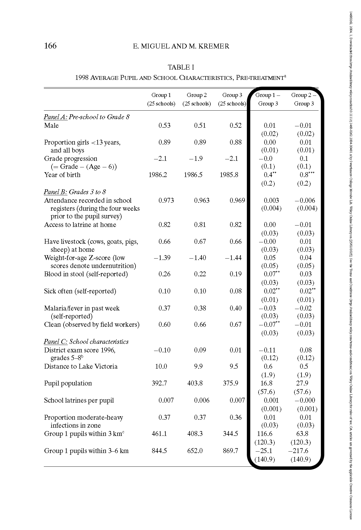{.width=200%}

School Participation

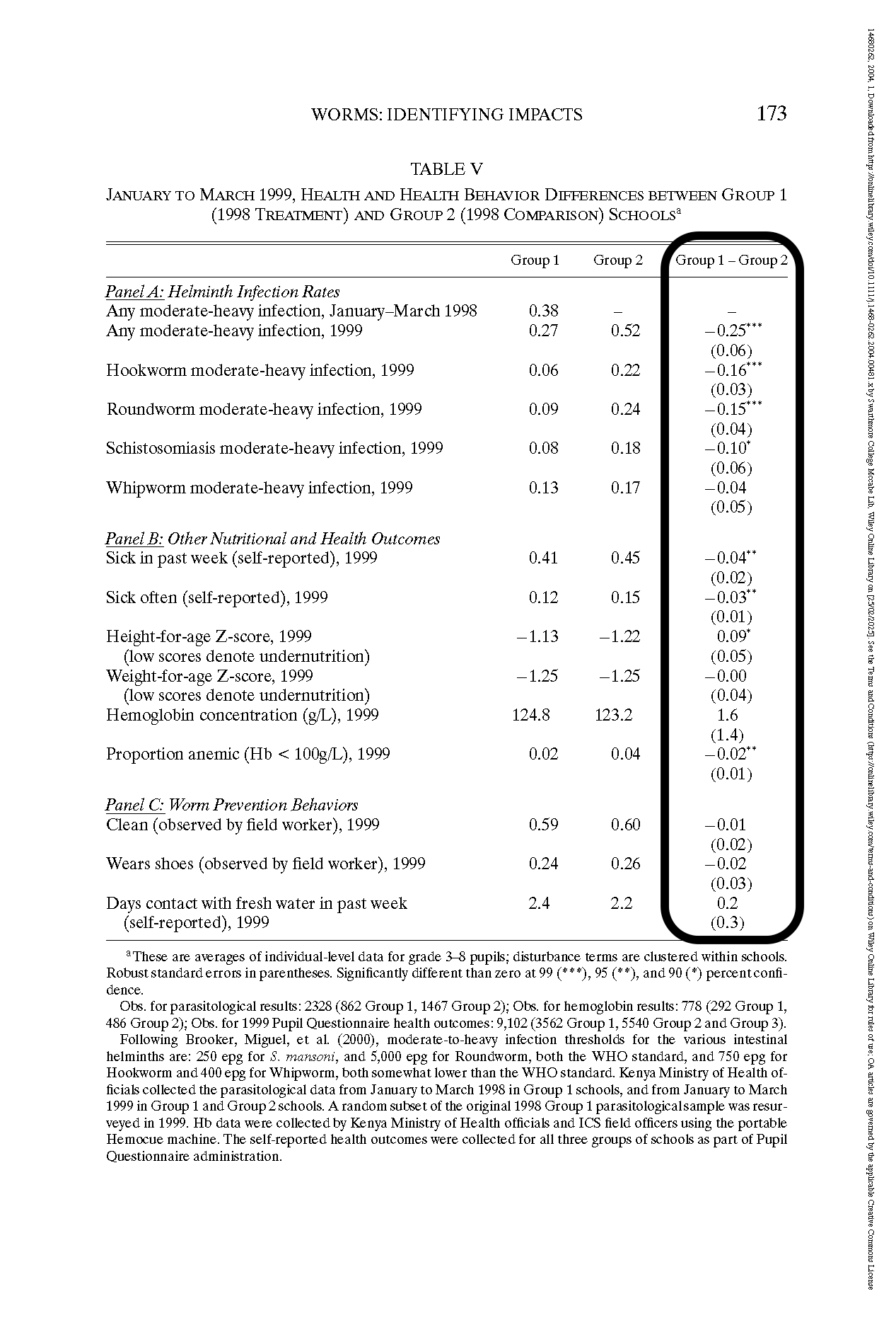{.width=200%}

Matched Sampling

With a matched sample, you can compare the means of the treatment and control groups
Or perhaps it shows the effects of the same unit before and after treatment
This design often leads to a smaller sampling error than the independent-sample design because variation between sampled items is eliminated as a source of sampling error.

Example

A state government wants to evaluate two different job training programs for unemployed workers. They randomly assigned participants to either Program A or Program B, and then tracked their employment outcomes over 6 months.

To control for individual characteristics, they matched participants across the programs based on factors like age, education level, and prior work experience - with each participant in Program A having a matched counterpart in Program B. The government wants to determine if there is a difference in mean employment rates between the two programs. Use a 0.05 level of significance to analyze the data shown in the next slide.

Example

Participant Pair	Employment Success (Months)
	Program A	Program B	Difference
Pair 1	32	25	7
Pair 2	30	24	6
Pair 3	19	15	4
Pair 4	16	15	1
Pair 5	15	13	2
Pair 6	18	15	3
Pair 7	14	15	-1
Pair 8	10	8	2
Pair 9	7	9	-2
Pair 10	16	11	5

Example

In this case, we can calculate the mean of the difference:

\[ \bar{d} = \bar{X}_t - \bar{X}_c = \frac{7 + 6 + 4 + 1 + 2 + 3 - 1 + 2 - 2 + 5}{10} = 2.7 \]

The standard deviation of the difference is:

\[ s = \sqrt{\frac{\sum{(d_i - \bar{d})^2}}{n-1}} = 2.9 \]

Example

The hypotheses are:

\[ H_0: \mu_d = 0 \]

\[ H_1: \mu_d \neq 0 \]

The level of significant is 0.05

The test statistic is:

\[ \frac{\bar{d} - \mu_d}{s/\sqrt{n}} = \frac{2.7-0}{2.9/\sqrt{10}} = 2.94 \]

The critical value is: T-TABLE

Since $2.94 > 2.262$, we reject the null hypothesis.

Proportions

We can also test differences in proportions.
We can use the normal distributions as long as

\[ np_1 \geq 5 \]

\[ n(1-p_1) \geq 5 \]

\[ np_2 \geq 5 \]

\[ n(1-p_2) \geq 5 \]

Interval Estimate

The confidence interval for the difference in proportions is:

\[ (p_1 - p_2) \pm z_{\alpha/2}\sqrt{\frac{p_1(1-p_1)}{n_1} + \frac{p_2(1-p_2)}{n_2}} \]

Hypothesis Tests (for no difference)

The null hypothesis for a two-tailed test is:

\[ H_0: p_1 - p_2 = D_0 \]

The alternative hypothesis is:

\[ H_1: p_1 - p_2 \neq D_0 \]

For a right-tailed test:

\[ H_0: p_1 - p_2 <= D_0 \]

\[ H_1: p_1 - p_2 > D_0 \]

For a left-tailed test:

\[ H_0: p_1 - p_2 >= D_0 \]

\[ H_1: p_1 - p_2 < D_0 \]

Tests for Equality

For each of these tests, we are testing for equality of proportions, meaning our null hypothesis assumes that $p_1 = p_2=p$.

The standard error under this assumption is:

\[ \sqrt{p(1-p)(\frac{1}{n_1} + \frac{1}{n_2})} \]

And the pooled estimator is a weighted estimate of the different proportions by their sample size:

\[ \bar{p} = \frac{n_1p_1 + n_2p_2}{n_1 + n_2} \]

Giving us a test statistic:

\[ \frac{p_1 - p_2}{\sqrt{\bar{p}(1-\bar{p})(\frac{1}{n_1} + \frac{1}{n_2})}} \]

Example

Market Research Associates is conducting research to evaluate the effectiveness of a client’s new advertising campaign. Before the new campaign began, a telephone survey of 150 households in the test market area showed 60 households “aware” of the client’s product (0.4). The new campaign has been initiated with TV and newspaper advertisements running for three weeks.

A survey conducted immediately after the new campaign showed 120 of 250 households “aware” of the client’s product (0.48). Can we conclude, using a 0.05 level of significance, that the proportion of households aware of the client’s product increased after the new advertising campaign?

Example

The null hypothesis is:

\[ H_0: p_1 - p_2 \leq 0 \]

\[ H_1: p_1 - p_2 > 0 \]

The test statistic is:

\[ \bar{p}=\frac{250(.48)+150(.40)}{250+150}=\frac{180}{400}=.45 \]

\[ s_{\bar{p}_1-\bar{p}_2}=\sqrt{.45(.55)\left(\frac{1}{250}+\frac{1}{150}\right)}=.0514 \]

\[ z=\frac{(.48-.40)}{.0514}=\frac{.08}{.0514}=1.56 \]

The p-value would be defined by:

\[ P(Z > 1.56) = 1 - P(Z < 1.56) = 1 - .9406 = .0594 \]

Since the p-value is greater than 0.05, we fail to reject the null hypothesis.

Inference about Means with Two Populations

Agenda

Difference in Means

Difference in Means

Difference in Means

Difference in Means

Central Limit Theorem

The Variance of the Difference in Means

Difference in Means

Confidence Intervals

Two-tailed Tests

One-tailed tests

\(\sigma\) Unknown

The t-distribution

Degrees of Freedom

Example:

Example:

Example:

Example:

Example:

Example:

Example:

Example:

Confidence Intervals not Crossing

Example:

Example:

Summary

Example: Deworming

Economic & Policy Implications

The Study (Kenya, 1998-2001)

Treatment

Results

Checking for Balance

Checking for Balance

School Participation

Matched Sampling

Example

Example

Example

Example

Proportions

Interval Estimate

Hypothesis Tests (for no difference)

Tests for Equality

Example

Example