We talked a little about this in the beginning of the course.
For this class, we will explore two ways to think about causality:
DAGS
Potential Outcomes
Both present a way to think about causality in terms of counterfactuals.
Specifically, a causal effect is defined as a comparison between two states of the world:
One state where an intervention was applied, and another state where it wasn’t
One is more visual and the other, more mathy…
DAGs and potential outcomes are different ways to think about the same thing.
Potential outcomes might be a better way to express selection bias and the fundamental problem of causal inference.
But DAGs are an intuitive way to think about causal relationships and are great for understanding omitted variable bias and confounding.
But each can be expressed in terms of the other.
What are Directed Acyclic Graphs (DAGs)?
A directed acyclic graph (DAG) is a finite directed graph with no directed cycles.
A directed graph is a way to represent a set of objects connected by edges, where the edges have a direction.
The direction of the edges indicates the direction of the relationship between the objects.
Specifically, the causal relationship.
Acyclic means that there are no cycles in the graph, i.e., it is not possible to start at one node and follow a sequence of edges that leads back to the same node.
DAGs are often used to represent causal relationships between variables in a system.
Connection to Causality
DAGS represent a world of causality where one thing affects another in one direction.
Represents a chain of causal relationships.
The causal effects represent some underlying unobserved process.
So DAGS are powerful, but they aren’t good at representing things such as:
Reverse Causality
Simultaneity
Causal Effects
Causal Effects can happen in two ways:
Direct:
flowchart LR
    D --> Y
Mediated (indirect):
flowchart LR
    D --> X --> Y
A DAG represents the full set of causal relationships in a system and their effect on Y, the outcome
Which also means that a lack of an arrow explicitly means that there is no causal relationship between the two variables.
The Causal Model
Where does the DAG come from?
A DAG is a theoretical representation of the state-of-the-art knowledge about the phenomena you’re studying.
It’s what an expert would say is the thing itself, and that expertise comes from a variety of sources.
Examples include economic theory, other scientific models, conversations with experts, your own observations and experiences, literature reviews, as well as your own intuition and hypotheses.
Why?
Causality and understanding causal relationships cannot be a one-size-fits-all approach or one that can be “discovered” in the data.
DAGs are very helpful for communicating research designs and estimators
Through concepts such as the backdoor criterion and collider bias, a well-designed DAG can help you develop a credible research design for identifying the causal effects of some intervention.
And finally, DAGs drive home the point that assumptions are necessary for any and all identification of causal effects
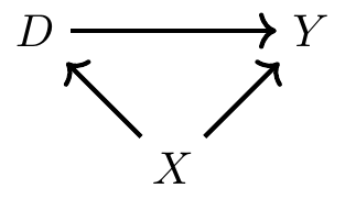
A simple example
Three random variables: \(X\), \(Y\), and \(D\).
A direct path from \(D\) to \(Y\).
A direct path from \(X\) to \(Y\).
But also \(D \leftarrow X \to Y\).
A “backdoor” path.
Not a causal path.
The backdoor path is a confounding path.
Creates a spurious correlation between \(D\) and \(Y\).
Similar to “omitted variable bias” in regression.
What is omitted variable bias?
Omitted variable bias is a type of bias that occurs when a model does not include one or more relevant variables.
This can lead to biased estimates of the causal effect of the included variables on the outcome variable.
If our true model is:
\[
Y = \beta_0 + \beta_1 D + \beta_2 X + \varepsilon
\]
But suppose you run a “naive” regression:
\[
Y = \tilde{\beta}_0 + \tilde{\beta}_1 D + \tilde{\varepsilon}
\]
Then \(\tilde{\varepsilon} = \beta_2 X + \epsilon\).
Back to DAGs
Not controlling for \(X\) creates a “backdoor” path from \(D\) to \(Y\).
\(X\) is a confounder.
Also a “noncollider”.
A noncollider is a variable that is not a common effect of two other variables.
We call \(X\) a confounder because it is a common cause of \(D\) and \(Y\).
Sometimes \(D\) takes different values and causes changes in \(Y\)
But sometimes \(D\) takes different values and \(Y\) changes because of \(X\).
If we could “control” for \(X\), we could eliminate the backdoor path.
Because our OLS regression would calculate \(b_1\) such that we would take into account the effect of \(X\) on \(Y\) and \(X\) on \(D\).
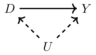
Unobserved Confounder
What if the confounder between \(D\) and \(Y\) is unobserved?
In this case, we show the confounder as a dashed line.
\(U\) is a unobserved confounder.
It exists, but may not be measurable, or is missing from the data.
This backdoor path is open.
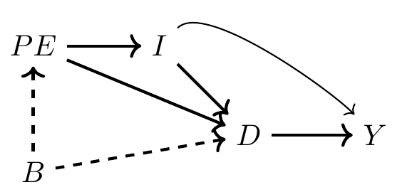
More Realistic Example
Does college education cause higher earnings?
According to Becker, education increases the marginal product of labor, and since markets pay their marginal product, education increases earnings.
But college education is not randomly assigned.
Chosen based on subjective preferences and resource constraints.
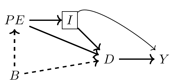
Here, \(D\) is college education, \(Y\) is earnings, \(PE\) be parental education, \(I\) is family income, \(B\) are unobserved background factors such as ability.
What do you think this of this DAG? Do you agree with it? Is there something missing?
Each person has some background. It’s not contained in most data sets, as it measures things like intelligence, contentiousness, mood stability, motivation, family dynamics, and other environmental factors. Hence, it is unobserved in the picture. Those environmental factors are likely correlated between parent and child and therefore subsumed in the variable \(B\).
Background causes a child’s parent to choose her own optimal level of education, and that choice also causes the child to choose their level of education through a variety of channels. First, there is the shared background factors, \(B\). Those background factors cause the child to choose a level of education, just as her parent had. Second, there’s a direct effect, perhaps through simple modeling of achievement or setting expectations, a kind of peer effect. And third, there’s the effect that parental education has on family earnings, \(I\), which in turn affects how much schooling the child receives. Family earnings may itself affect the child’s future earnings through bequests and other transfers, as well as external investments in the child’s productivity.
DAGs also tell us what IS NOT Happening
No direct from \(B\) to \(Y\), except through schooling.
That’s an assumption
And you are free to call foul on this assumption if you think that background factors affect both schooling and the child’s own productivity
Next Steps
List all direct and indirect paths:
\(D \rightarrow Y\) (the causal effect of education on earnings)
\(D \leftarrow I \rightarrow Y\) (the effect of family income on earnings, through education, backdoor path 1)
\(D \leftarrow PE \rightarrow I \rightarrow Y\) (the effect of parental education on earnings, through family income, and education, backdoor path 2)
\(D \leftarrow B \rightarrow PE \rightarrow I \rightarrow Y\) (the effect of background on earnings, through parental education, through family income, and education, backdoor path 3)
Four paths between \(D\) and \(Y\).
One direct path and three backdoor paths
Since none of them are colliders, the paths are all open.
Open backdoor paths is that they create systematic and independent correlations between \(D\) and \(Y\).
Put a different way, the presence of open backdoor paths introduces bias when comparing educated and less-educated workers.
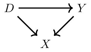
Colliding
But what is a collider?
So the paths are now:
\(D \rightarrow Y\) (the direct effect)
\(D \rightarrow X \leftarrow Y\) (backdoor path)
Colliders are special in part because when they appear along a backdoor path, that backdoor path is closed simply because of their presence.
Colliders, when they are left alone, always close a specific backdoor path.
Backdoor Criterion
Open backdoor paths create omitted variable bias.
Closed backdoor paths do not create omitted variable bias.
Our goal is to close the backdoor paths.
Two ways:
You can condition on the confounder (control for that variable)
Or you can close it through the appearance of a collider.
By not conditioning on a collider, you will have closed that backdoor path and that takes you closer to your larger ambition to isolate some causal effect.
Controlling for Confounders
When all backdoors are closed, then you have satisfied the backdoor criterion.
A set of variables satisfies the backdoor criterion in a DAG if and only if \(X\) blocks every path between confounders that contain an arrow from \(D\) to \(Y\)
Back to the Example
The backdoor criterion is a way to identify confounding variables in a DAG. In this case, \(I\) is a non-collider along every backdoor path.
By conditioning on \(I\), we can close the backdoor paths and isolate the causal effect of \(D\) on \(Y\).
By conditioning/controlling \(I\), \(D\) takes on a causal interpretation.
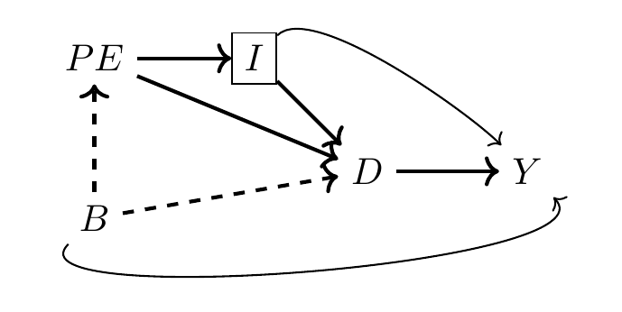
Calling the DAG into question
But what if that DAG is not satisfying…
What if \(B\), or background has a direct effect on \(Y\)?
In this case, \(B\) is a confounder.
And we don’t know the nature of \(B\) because it is an unobserved variable.
So we can’t condition on it.
So we can’t close the backdoor path.
So we can’t isolate the causal effect of \(D\) on \(Y\).
Why shouldn’t we condition on colliders?
Conditioning on a collider opens up a backdoor path.
Why?
Because conditioning on a collider creates a correlation between the two variables that are not otherwise correlated.
Intuition: If you condition on a variable that is a common effect of two other variables, you are creating a correlation between those two variables that is not otherwise there.
Same as the idea that if two variables are independent, conditioning on a third variable might create a correlation between them.
Example: Discrimination and Collider Bias
Gender Discrimination in labor markets
Age-old explanation that gender discrimination does not exist: Once we account for factors such as location, tenure, job role, level, performance, time off etc…, there is no longer any difference in pay between men and women.
But what if discrimination is through occupational sorting?
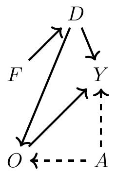
If discrimination leads to women taking lower quality and lower-paying jobs, then accounting for occupation is actually a collider!
D -> discrimination
O -> occupation
Y -> earnings
F -> female ==1
A -> ability
What are the paths?
\(D \rightarrow O \rightarrow Y\) (discrimination affects occupation, which affects earnings)
\(D \rightarrow O \leftarrow A \rightarrow Y\) (discrimination affects occupation, and so does ability, which affects earnings)
The first is not a backdoor path, but rather what’s called a “mediation”
Discrimination is “mediated” through occupation before it affects earnings.
This would imply that women are discriminated against, which in turn affects which jobs they hold, and as a result of holding marginally worse jobs, women are paid less.
The second path relates to that channel but is slightly more complicated. In this path, unobserved ability affects both which jobs people get and their earnings.
Our Regression
If we just run the following regression:
\[
Y_i = \alpha + \beta D_i + \varepsilon_i
\]
\(\beta\) will yield the total effect as a combination of the direct effect and the mediated effect through occupation.
But if we wanted to condition on occupation, so that we could compare men and women in similar jobs:
In this case, we close the mediation channel, but conditioning on \(O\) opens the backdoor path because it is a collider!
We’ve now created correlation between discrimination and ability!
Why?
By conditioning on occupation, we are looking at the effect of discrimination within an occupation, where discrimination and ability confound each other.
We don’t know whether within an occupation, earnings are being driven by discrimination or by differences in ability.
What we need to control for then is occupation and ability.
But we don’t know the nature of ability, so we can’t condition on it.
clear all
set obs 10000

* Half of the population is female.
generate female = runiform()>=0.5

* Innate ability is independent of gender.
generate ability = rnormal()

* All women experience discrimination.
generate discrimination = female

* Data generating processes
// occupation is a function of ability,  and discrimination as in DAG
generate occupation = (1) + (2)*ability + (0)*female + (-2)*discrimination + rnormal()
generate wage = (1) + (-1)*discrimination + (1)*occupation + 2*ability + rnormal()

* Regressions
regress wage discrimination
regress wage discrimination occupation
regress wage discrimination occupation ability
Lessons from Colliders: Bad Controls
Econometrics in many cases takes a “kitchen sink” approach to regression.
The idea is that the more controls you have, the better your estimate of the causal effect.
But this is not true.
Conditioning on a collider can open up backdoor paths and create spurious correlations.
This is a form of “bad control”.
Bad controls are variables that are not causally related to the outcome variable, but are included in the model anyway.
Bad controls can create bias in the estimates of the causal effect of the included variables on the outcome variable.
Colliders as Sample Selection
Sample selection is a form of collider bias.
When we condition on a sample that is not representative of the population, we are conditioning on a collider.
This can create spurious correlations between the variables in the sample.
We will talk about sample selection in more detail later in the course.
What do DAGs teach us?
Causality and causal inference is not a one-size-fits-all approach.
It is not something that more data can solve.
Causation is about understanding the underlying processes that drive the relationships between variables.
It involves creating a model of the system
And therefore, all causal arguments require assumptions.